Announcements & Reminders
March 11, next Monday is the first online test (10% of final grade)
8:00 in the morning till 23:59
Take only once, will need 30 min
Will automatically submit after 30 min
Compulsory!
Will cover materials up to and including this lecture
You will get email notification from Wattle
There will be a practice test to help you familiarize yourself with the system
📖 Mappings: functions and correspondences#
⏱ | words
Sources and reading guide#
Sources and reading guide
[Sydsæter, Hammond, Strøm, and Carvajal, 2016]
Chapters 4, 5, 9.6 (pp. 350-351 only), 11.1, and 11.5.
Introductory mathematical economics references:
[Haeussler Jr and Paul, 1987]: Chapters 0, 3, 4, 5, and 17.1.
[Shannon, 1995]: Chapters 1, 2, and 6.
Advanced high school references:
[Coroneos, n.d.]: Chapters 1, 2, 4, and 7.
[Coroneos, n.d.]: Chapters 1 and 2.
Introductory mathematics references:
[Adams and Essex, 2018]: Chapters P, 3, and 11.
[Kline, 1967]: pp. 419–432.
[Silverman, 1969]: Chapters 7 and 14.
[Spivak, 2006]: Chapters 1, 2, 3, 4, 16, 18, and 19.
[Thomas Jr and Finney, 1996]: Chapters P, 6, and 12.
More advanced references:
[Corbae, Stinchcombe, and Zeman, 2009]: Chapter 2 (pp. 15-71).
[Kolmogorov and Fomin, 1970]: Chapter 1 (pp. 1-36).
[Simon and Blume, 1994]: Chapters 2 and 13 (pp. 10-38 and 273-299).
The following websites contain discussions of the concept of relatively prime, or co-prime, numbers and polynomials. This is relevant to the topic of rational functions and partial fractions.
Mappings#
Definition
Let \(X\) and \(Y\) be two sets. A rule \(f\) that assigns one or more elements of \(Y\) to each element of \(X\) is called a mapping from \(X\) into \(Y\). It is denoted by \(f: X \rightarrow Y\).
Definition
The set \(X\) is known as the domain of the mapping \(f\). The mapping must be defined for every element of \(X\). This means that \(x \in X \implies f(x) \in Y\).
Definition
The set \(Y\) is known as the co-domain of the mapping \(f\). Mappings are not required to generate \(Y\) from \(X\). This means that there might exist one or more elements \(y \in Y\) such that \(y \ne f(x)\) for any \(x \in X\).
Definition
The set of values \(y \in Y\) that can be generated from \(X\) by the function \(f\) is known as the image of \(X\) under \(f\). Sometimes the image of \(X\) under \(f\) is referred to as the range of \(f\). We will denote the range of \(f\) by \(f(X)\).
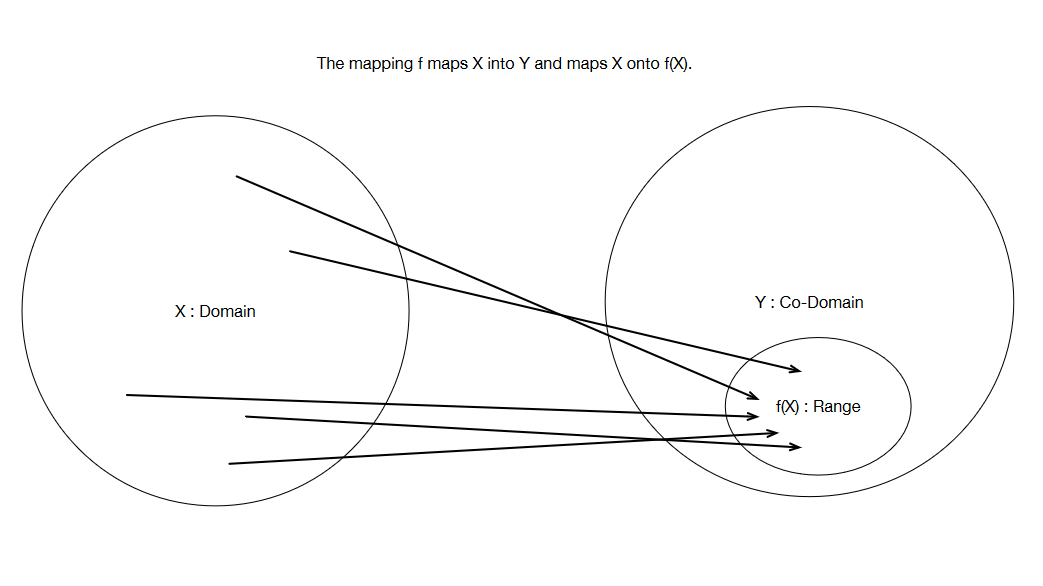
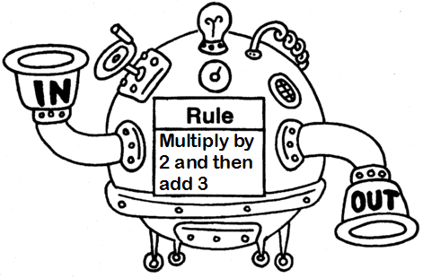
Fig. 13 Diagrammatic representation of a mapping#
Images#
Consider a mapping \(f: X \rightarrow Y\). The image of the point \(x \in X\) under the mapping \(f\) is the point, or collection of points, given by \(f(x) \in Y\).
The image of the set \(A \subseteq X\) under the mapping \(f\) is the set \(f(A) = \{f(x) \in Y : x \in A\}\).
Clearly \(f(A) \subseteq Y\).
The image of the domain (\(X\)) under \(f\) is the set \(f(X) = \{f(x) \in Y : x \in X \}\) referred to as the range of \(f\).
Clearly \(f(X) \subseteq Y\).
Note that if \(f: X \rightarrow Y\) and \(A \subseteq X\), then \(f(A) \subseteq f(X) \subseteq Y\).
Pre-images#
Consider a mapping \(f: X \rightarrow Y\).
The pre-image of the point \(y \in Y\) under the mapping \(f\) is the point, or collection of points, in \(X\) for which \(y = f(x)\).
It is possible for a point \(y \in Y\) to have either
no pre-image
a unique pre-image, or
multiple pre-images.
Note
The term multiple (image and pre-image) is equivalent to pre-image be a set of muliple points.
If a point \(y \in Y\) has a unique pre-image under the mapping \(f\), then it is denoted by \(f^{−1}(y)\).
The pre-image of the set \(B \subseteq Y\) under \(f\) is the set \(f^{−1}(B) = \{x \in X : f(x) \in B\}\).
Recall that it is possible for there to exist \(y \in Y\) such that \(y \ne f(x)\) for any \(x \in X\). If the set B consists entirely of such points, then \(f^{−1}(B) = \varnothing\).
Since \(f(x) \in Y\) for all \(x \in X\), it must be the case that \(f^{-1}(Y) = X\).
Types of mappings#
There are four basic types of mappings. These are as follows.
A one-to-one mapping:
Each point in \(X\) has a unique image in \(Y\); and
Each point in \(Y\) has either a unique pre-image in \(X\) or no pre-image in \(X\).
example: \(f(x) = x\)
A many-to-one mapping:
Each point in \(X\) has a unique image in \(Y\); but
At least one point in \(Y\) has multiple pre-images in \(X\).
example: \(f(x) = x^2\)
A one-to-many mapping:
At least one point in \(X\) has multiple images in \(Y\); but
Each point in \(Y\) has either a unique pre-image in \(X\) or no pre-image in \(X\).
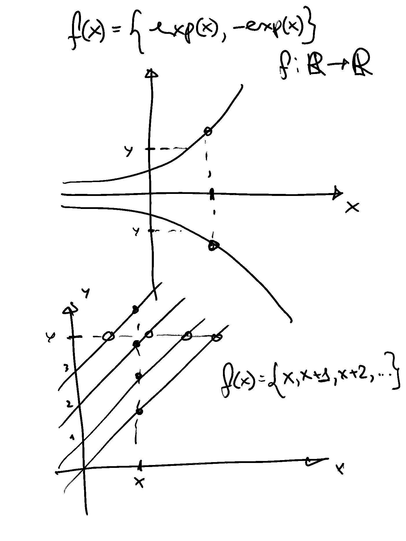
example: \(f(x) = \{e^x,-e^x\}\)
A many-to-many mapping:
At least one point in \(X\) has multiple images in \(Y\); and
At least one point in \(Y\) has multiple pre-images in \(X\).
example: \(f(x) = \{x,x+1,x+2,\dots\}\)
Definition
Mappings whose domain points all have unique images are known as functions. In other words, one-to-one mappings and many-to-one mappings are known as functions.
Definition
Mappings that have at least one domain point with multiple images are known as correspondences. In other words, one-to-many mappings and many-to-many mappings are known as correspondences.
Note that we could express a correspondence of the form \(f : X \rightarrow Y\) as a function of the form \(g: X \rightarrow 2^Y\).
Into and onto#
Consider a mapping \(f : X \rightarrow Y\). Clearly we must have \(f(X) \subseteq Y\) (range is a subset of co-domain).
If \(f(X ) \subset Y\), so that \(f(X) \ne Y\), we say that \(f\) maps \(X\) “into” \(Y\).
If \(f(X) = Y\), we say that \(f\) maps \(X\) “onto” \(Y\).
Definition
If \(f(X) = Y\) and \(f\) is a function, then we call \(f\) a surjection.
One-to-one#
Definition
A one-to-one function \(f: X \rightarrow Y\) is called an injection. The pre-image of a one-to-one function is known as its inverse.
Fact
A function \(f : X \rightarrow Y\) is one-to-one if
The contra-positive version of this condition is that
Examples:
\(f : \mathbb{R} \rightarrow \mathbb{R}\) defined by \(f(x ) = x\) is a one-to-one function.
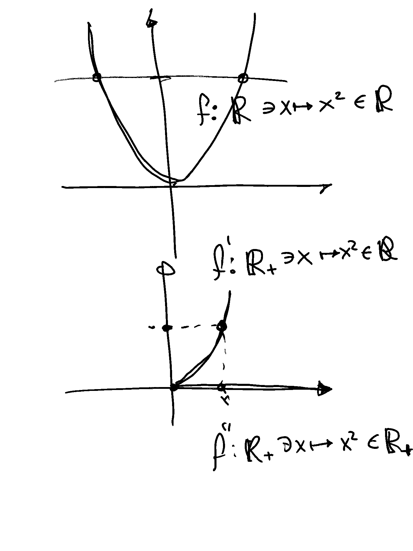
\(f : \mathbb{R} \rightarrow \mathbb{R}\) defined by \(f(x ) = x^2\) is not a one-to-one function.
\(f : \mathbb{R}_+ \rightarrow \mathbb{R}\) defined by \(f(x) = x^2\) is a one-to-one function.
Example
Consider the mapping \(f: \mathbb{R} \rightarrow \mathbb{R}\) defined by \(f(x) = x\). This is sometimes called the identity map. Note that \(f\) is both onto and one-to-one. This means that \(f\) is a bijection. It also means that the pre-image of \(f\) is an inverse function.
Definition
A mapping that is both an injection and a surjection is called a bijection. In other words, a function that is both one-to-one and onto is called a bijection.
Fact
If \(f: X \to Y\) a bijection, then there exists a unique function \(\phi: Y \to X\) such that
That function \(\phi\) is called the inverse of \(f\) and written \(f^{-1}\)

Example
Consider the mapping \(f: \mathbb{R} \rightarrow \mathbb{R}\) defined by \(f(x) = x^2\). Note that \(f\) is into, but not onto, because \(f^{−1}(\mathbb{R}_{−−}) = \varnothing\), where \(\mathbb{R}_{−−} = \{x \in \mathbb{R} : x < 0\}\).
Note also that \(f\) is many-to-one, and hence not one-to-one, because \(2 \in \mathbb{R}, (−2) \in \mathbb{R}, 2 \ne (−2)\), and both \(2^2 = 4\) and \((−2)^2 = 4\). This means that \(f\) is neither an injection nor a surjection. Thus it cannot be a bijection. It also means that the pre-image of \(f\) is not an inverse function.
Composite functions#
Definition
Let \(f : X \rightarrow Y\) and \(g : Y \rightarrow Z\) be functions. The composite function \(h = g \circ f\) is defined by \(h(x) = g(f(x))\). The composite function \(h = g \circ f\) is a mapping \(h : X \rightarrow Z\).
Example
Let \(f : \mathbb{R}^2_{++} \rightarrow \mathbb{R}_{++}\) be defined by \(f(x_1, x_2) = x_1^\alpha \; x_2^{(1 − \alpha)}\) for some fixed \(\alpha \in (0, 1)\).
Let \(g : \mathbb{R}_{++} \rightarrow \mathbb{R}\) be defined by \(g(x) = ln(x)\).
Then the composite function \(h = g \circ f\) is a mapping \(h: \mathbb{R}^2_{++} \rightarrow \mathbb{R}\) that is defined by \(h(x_1, x_2) = g(f(x_1, x_2)) = ln(x_1^\alpha \; x_2^{(1 − \alpha)}) = \alpha \; ln(x_1) + (1 − \alpha) \; ln(x_2)\)
Non-decreasing and strictly increasing functions#
Definition
A function \(f : X \rightarrow \mathbb{R}\), where \(X \subseteq \mathbb{R}\), is said to be a non-decreasing function if
Definition
A function \(f : X \rightarrow \mathbb{R}\), where \(X \subseteq \mathbb{R}\), is said to be a strictly increasing function if both
(a) \(x = y \iff f(x) = f(y)\); and
(b) \(x < y \iff f(x) < f(y)\).
Note the following:
A strictly increasing function is also a one-to-one function.
There are some one-to-one functions that are not strictly increasing.
A strictly increasing function is also a non-decreasing function.
There are some non-decreasing functions that are not strictly increasing.
Exercise: give examples of each case
Definition
Non-increasing and strictly decreasing functions are defined in a similar manner, with the inequality signs flipped.
Utility function and preference relationship#
Suppose that \(U : X \rightarrow \mathbb{R}\) is a utility function that represents the weak preference relation \(\succsim\). This means that \(x \succsim y \iff U(x) \geqslant U(y)\).
Let \(f: \mathbb{R} \rightarrow \mathbb{R}\) be a strictly increasing function. Consider the composite function \(V = f \circ U\). It can be shown that \(V\) is also a utility function that represents the weak preference relation \(\succsim\). In other words, it can be shown that \(x \succsim y \iff V(x) \geqslant V(y)\).
Definition
Monotonic transformation of a given function is its composition with a a strictly increasing or strictly decreasing function.
Fact
Monotonic transformation of a utility function that represents a preference relation will represent the same preference relation.
Example
Consider a consumer whose preferences over bundles of strictly positive amounts of each of two commodities can be represented by a utility function \(U : \mathbb{R}^2_{++} \rightarrow \mathbb{R}_{++}\) of the form
where \(A > 0, \alpha > 0\), and \(\beta > 0\).
Such preferences are known as Cobb-Douglas preferences.
The function \(f: \mathbb{R}_{++} \rightarrow \mathbb{R}_{++}\) defined by \(f(x) = \left( \frac{1}{A} \right)x\) is strictly increasing. Thus we know that another utility function that represents this consumer’s preferences is
The function \(g: \mathbb{R}_{++} \rightarrow \mathbb{R}_{++}\) defined by \(g(x) = x^{\frac{1}{(\alpha + \beta)}}\) is strictly increasing. (If any relevant surd expression can be either positive or negative, then we will assume that the positive option is chosen throughout this Cobb-Douglas preferences example.) Thus we know that another utility function that represents this consumer’s preferences is
where \( \gamma = \frac{\alpha}{\alpha + \beta} \in (0, 1)\).
The function \(k: \mathbb{R}_{++} \rightarrow \mathbb{R}\) defined by \(k(x) = ln(x )\) is strictly increasing. Thus we know that another utility function that represents this consumer’s preferences is
Graphs#
Definition
A graph of a mapping \(f \colon X \to Y\) is a set \(\Gamma \subset X \times Y\) of points \(x \in X\) and \(y \in Y\) where it holds \(y \in f(x)\), or \(y = f(x)\) in hte case \(f\) is a function.
For the functions \(\mathbb{R} \to \mathbb{R}\) a graph can be conveniently drawn on a plane. We can also easily plot graphs of correspondences \(\mathbb{R} \to 2^\mathbb{R}\).
Shifting the graph#
Fact
Consider \(\Gamma_0\) the graph of function \(f(x): \mathbb{R} \to \mathbb{R}\). Denote \(\Gamma_1\) the graph of the composite function \(g(x) = af(bx+c)+d\), such that when \(a=b=1\) and \(c=d=0\) \(f(x)=g(x)\). It holds that:
for \(a \ne 1\), \(a>0\) graph \(\Gamma_1\) is a vertical stretch or compression of \(\Gamma_0\) by a factor of \(|a|\)
for \(a<0\) in addition graph \(\Gamma_1\) flips around the horizontal axis
for \(b \ne 1\), \(b>0\) graph \(\Gamma_1\) is a horizontal stretch or compression of \(\Gamma_0\) by a factor of \(|b|\)
for \(b<0\) in addition graph \(\Gamma_1\) flips around the vertical axis
for \(c \ne 0\) graph \(\Gamma_1\) is a horizontal shift of \(\Gamma_0\) by \(\frac{c}{b}\), left for \(\frac{c}{b}>0\) and right for \(\frac{c}{b}<0\)
for \(d \ne 0\) graph \(\Gamma_1\) is a vertical shift of \(\Gamma_0\) by \(d\), up for \(d>0\) and down for \(d<0\)
Example
Online graphing tools like Desmos
Graph of the inverse function#
Fact
When the inverse exists, its graph is a flip of the original graph over the 45 degree line.
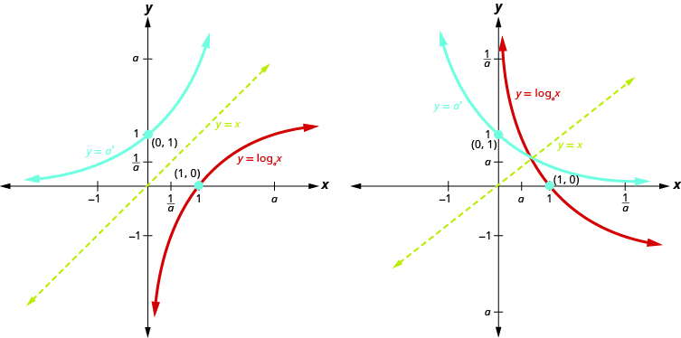
Fig. 16 Graph of inverse functions#
Some types of functions#
Some types of univariate functions include the following:
Polynomial functions
These include constant functions, linear (and affine) functions, quadratic functions, and some power functions as special cases.
Exponentional functions
Power functions
Logarithmic functions
Trigonometric functions
We are unlikely to have enough time to cover trigonometric functions in this course. There are also multivariate versions of these types of functions.
Polynomial functions#
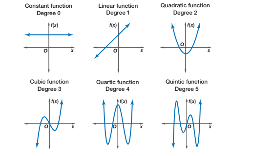
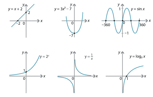
Fig. 17 Graphs of polynomial functions#
Definition
A polynomial function (of one variable) is a function of the form
In order to distinguish between different types of polynomials, we will typically assume that the coefficient on the term with the highest power of the variable \(x\) is non-zero. The only exception is the case in which this term involves \(x^0 = 1\), in which case we will allow both \(a_0 \ne 0\) and \(a_0 = 0\).
Example
A constant (degree zero) polynomial (\(a_0 \ne 0\) or \(a_0 = 0\)):
Example
A linear (degree one) polynomial (\(a_1 \ne 0\)):
It is sometimes useful to distinguish between linear functions and affine functions.
Example
A quadratic (degree two) polynomial (\(a_2 \ne 0\)):
Example
A cubic (degree three) polynomial (\(a_3 \ne 0\)):
Affine functions and linear functions#
Note that strict definition of a linear function \(f(x)\) requires \(f(\alpha x) = \alpha f(x)\) and \(f(x+y) = f(x) + f(y)\), where \(\alpha, x, y \in \mathbb{R}\).
However, we often loosely speak about a linear function of one variable being a function of the form \(f(x) = a_1 x + a_0\), where \(a_0 \in \mathbb{R}\) and \(a_1 \in \mathbb{R} \setminus \{0\}\) are fixed parameters, and \(x \in \mathbb{R}\) is the single variable.
Clearly, when \(a_0 \ne 0\), the definition of a linear function is not satisfied. In fact, it satisfies a different definition, that of an affine function. Strictly speaking, linear functions are thus \(f(x) = a_1 x\), in which \(a_0 = 0\).
Using this more precise terminology, the family of linear functions is a proper subset of the family of affine functions. Note that we assume that \(a_1 \in \mathbb{R} \setminus \{0\}\) in both cases.
Exponential functions#
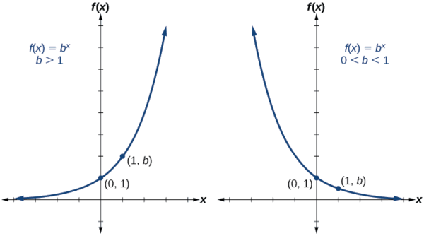
Fig. 18 Graphs of exponential functions#
Definition
An exponential function is a non-linear function in which the independent variable appears as an exponent.
where \(C\) is a fixed parameter (called the coefficient), \(a \in \mathbb{R}\) is a fixed parameter (called the base), and \(x \in \mathbb{R}\) is an independent variable (called the exponent).
Note that if \(a = 0\), then \(f(x)\) is only defined for \(x > 0\).
Note also that if \(a < 0\), then sometimes \(f(x) \notin \mathbb{R}\). An example of this is the case when \(C = 1, a = (−1)\) and \(x = \frac{1}{2}\). In this case, we have:
Popular choices of base#
Two popular choices of base for exponential functions are \(a = 10\) and \(a = e\), where \(e\) denotes Euler’s constant. Euler’s constant is defined to be the number
Note that Euler’s constant is an irrational number. This means that it is a real number that cannot be represented as the ratio of an integer to a natural number.
The function \(f(x) = e^x\) is sometimes called “the” exponential function.
Exponential arithmetic#
Assuming that the expressions are well-defined, we have the following laws of exponential arithmetic.
The power of zero: \(a^0 = 1\) if \(a \ne 0\), while \(a^0\) is undefined if \(a = 0\).
Multiplication of two exponential functions with the same base:
Division of two exponential functions with the same base:
An exponential function whose base is an exponential function:
Power functions#
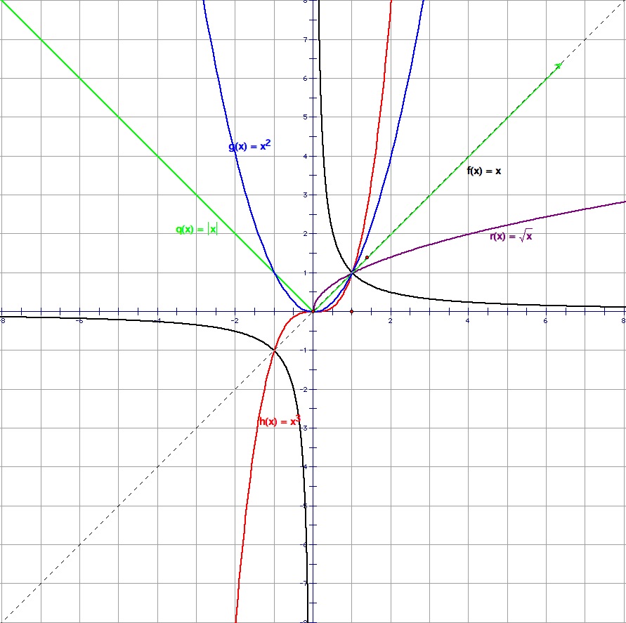
Fig. 19 Graphs of power functions#
Definition
A power function takes the form
where \(C \in \mathbb{R}\) is a fixed parameter, \(a \in \mathbb{R}\) is a fixed parameter, and \(x \in \mathbb{R}\) is an independent variable.
Note that when \(a \in \mathbb{N}\), a power function can also be viewed as a polynomial function with a single term.
Note that a power function can also be viewed as a type of exponential expression in which the base is \(x\) and the exponent is \(a\). This means that the laws of exponential arithmetic carry over to “power function arithmetic”.
Power function arithmetic#
Assuming that the expressions are well-defined, we have the following laws of power function arithmetic.
The power of zero: \(x^0 = 1\) if \(x \ne 0\), while \(x^0\) is undefined if \(x = 0\).
Multiplication of two power functions with the same base:
Division of two power functions with the same base:
A power function whose base is itself a power function:
A rectangular hyperbola#
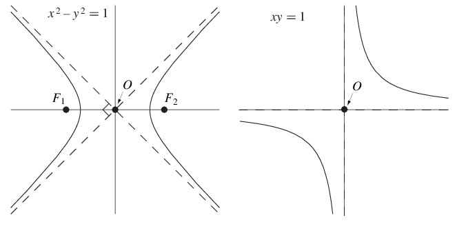
Fig. 20 Graphs of hyperbola#
Consider the function \(f : \mathbb{R} \setminus \{0\} \rightarrow \mathbb{R}\) defined by \(f(x) = \frac{a}{x}\), where \(a \ne 0\). This is a special type of power function, as can be seen by noting that it can be rewritten as \(f(x) = ax^{−1}\). The equation for the graph of this function is
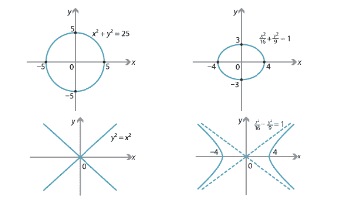
Note that this equation can be rewritten as \(xy = a\). This is the equation of a rectangular hyperbola.
Economic application: A constant “own-price elasticity of demand” demand curve.
Logarithms#
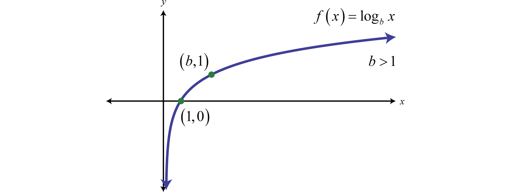
Fig. 21 Graphs of logarithmic function#
Definition
A logarithm function is the inverse of an exponent.
Thus we have
The expression \(log_a\) stands for “log base \(a\)” or “logarithm base \(a\)”. Popular choices of base are \(a = 10\) and \(a = e\).
The function
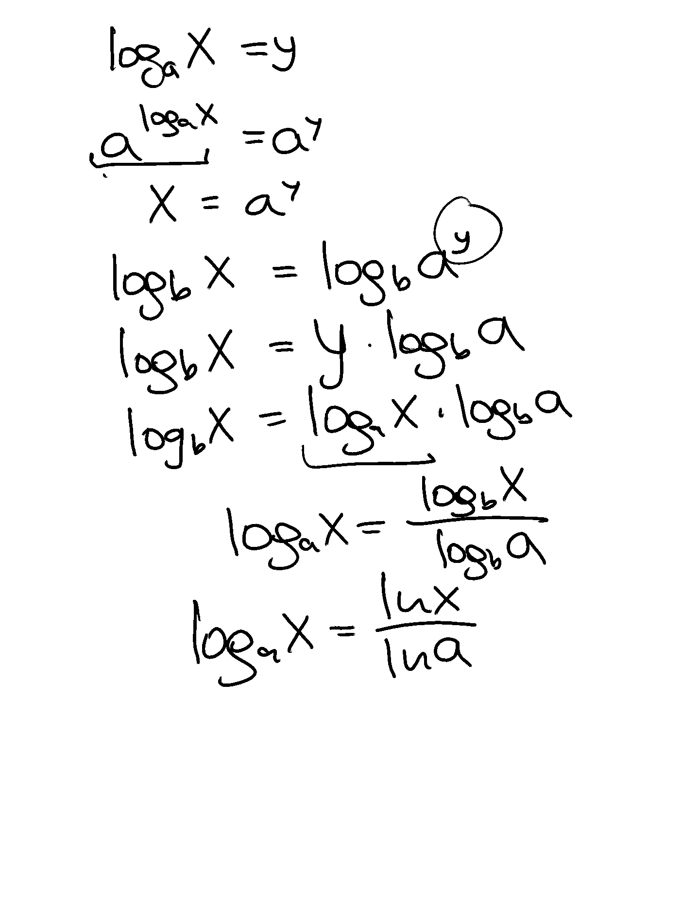
is the “logarithm base \(a\)” function. The “logarithm base \(a\)” function is the inverse for the “exponential base \(a\)” function. The reason for this is that
Natural (or Naperian) logarithms#
A “logarithm base e” is known as a natural, or Naperian, logarithm. It is named after John Napier. See Shannon (1995, pp. 270-271) for a brief introduction to John Napier. The standard notation for a natural logarithm is \(\ln\), although you could also use \(\log_e\).
The function
is the “logarithm base \(e\)” function. The natural logarithm function is the inverse function for “the” exponential function, since
Illustrate the inverse (or “reflection through the 45 degree (y = x) line”) relationship between ln (x ) and ex on the whiteboard.
Logarithmic arithmetic#
Assuming that the expressions are well-defined, we have the following laws of logarithmic arithmetic.
Multiplication of two logarithmic functions with the same base:
Division of two logarithmic functions with the same base:
A logarithmic function whose argument is an exponential function:
Note that
Rational functions#
Definition
A rational function \(R(x)\) is simply the ratio of two polynomial functions, \(P(x)\) and \(Q(x)\). It takes the form
where
is an \(m\)-th order polynomial (so that \(a_m \ne 0\)), and
is an \(n\)-th order polynomial (so that \(b_n \ne 0\)).
Note that there is no requirement that the polynomial functions \(P(x)\) and \(Q(x)\) be of the same order. (In other words, we do not require that \(m = n\).)
The most interesting case is when \(m < n\). In such cases, the rational function \(R(x)\) is called a “proper” rational function.
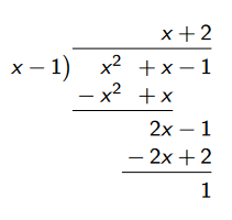
When \(m > n\), then we can always use the process of long division to write the original rational function \(R(x)\) as the sum of a polynomial function \(Y(x)\) and another proper rational function \(R^∗(x)\).
Some useful results about functions#
Fact
The pre-image of the union of two sets is equal to the union of the pre-images of each of the two sets: \(f^{−1}(A \cup B) = f^{−1}(A) \cup f^{−1}(B)\).
Proof
Let \(f: X \rightarrow Y\) and consider two sets, \(A \subseteq Y\) and \(B \subseteq Y\). We want to show that the pre-image of the union of two sets is equal to the union of the pre-images of each of the two sets: \(f^{−1}(A \cup B) = f^{−1}(A) \cup f^{−1}(B)\).
Note that
Example
Example: \(f: \mathbb{Z} \rightarrow \mathbb{R}\) defined by \(f(z) = z^2, A = [0, 9] \subset \mathbb{R}\), and \(B = [5, 25] \subset \mathbb{R}\). \(A \cup B = [0, 25] \subset \mathbb{R}\).
The pre-image mapping here is given by \(f^{−1}(y) = \pm \sqrt{y}\) if \(\pm \sqrt{y}\) is an integer, and \(f^{−1}(y) = \varnothing\) otherwise. Note that this pre-image mapping is not an inverse function, because \(\pm \sqrt{y}\) is sometimes multi-valued.
\(f^{−1}(A \cup B) = \{−5, −4, −3, −2, −1, 0, 1, 2, 3, 4, 5\}\)
\(f^{−1}(A) = \{−3, −2, −1, 0, 1, 2, 3\}\)
\(f^{−1}(B) = \{−5, −4, −3, 3, 4, 5\}\)
\(f^{−1}(A) \cup f^{-1}(B) = \{−5, −4, −3, −2, −1, 0, 1, 2, 3, 4, 5\} = f^{−1}(A \cup B)\)
Fact
The pre-image of the intersection of two sets is equal to the intersection of the pre-images of each of the two sets: \(f^{−1}(A \cap B) = f^{−1}(A) \cap f^{−1}(B)\).
Proof
Let \(f: X \rightarrow Y\) and consider two sets, \(A \subseteq Y\) and \(B \subseteq Y\). We want to show that the pre-image of the intersection of two sets is equal to the intersection of the pre-images of each of the two sets: \(f^{−1}(A \cap B) = f^{−1}(A) \cap f^{−1}(B)\).
Note that
Example
Example: \(f: \mathbb{Z} \rightarrow \mathbb{R}\) defined by \(f(z) = z^2, A = [0, 9] \subset \mathbb{R}\), and \(B = [5, 25] \subset \mathbb{R}\). \(A \cap B = [5, 9] \subset \mathbb{R}\).
The pre-image mapping here is given by \(f^{−1}(y) = \pm \sqrt{y}\) if \(\pm \sqrt{y}\) is an integer, and \(f^{−1}(y) = \varnothing\) otherwise. Note that this pre-image mapping is not an inverse function, because \(\pm \sqrt{y}\) is sometimes multi-valued.
\(f^{−1}(A \cap B) = \{−3, 3\}\)
\(f^{−1}(A) = \{−3, −2, −1, 0, 1, 2, 3\}\)
\(f^{−1}(B) = \{−5, −4, −3, 3, 4, 5\}\)
\(f^{−1}(A) \cap f^{-1}(B) = \{−3, 3\} = f^{−1}(A \cap B)\)
Fact
The image of the union of two sets is equal to the union of the images of each of the two sets: \(f(A \cup B) = f(A) \cup f(B)\).
Proof
Let \(f: X \rightarrow Y\) and consider two sets, \(A \subseteq Y\) and \(B \subseteq Y\). We want to show that the image of the union of two sets is equal to the union of the images of each of the two sets: \(f(A \cup B) = f(A) \cup f(B)\).
Note that
Example
Example: \(f: \mathbb{Z} \rightarrow \mathbb{R}\) defined by \(f(z) = z^2, A = \{1, 2, 3\} \subset \mathbb{Z}\), and \(B = \{2,3,4,5\} \subset \mathbb{Z}\).
\(A \cup B = \{1,2,3,4,5\} \subset \mathbb{Z}\)
\(f(A \cup B) = \{1, 4, 9, 16, 25\} \subset \mathbb{R}\)
\(f(A) = \{1, 4, 9\} \subset \mathbb{R}\)
\(f(B) = \{4, 9, 16, 25\} \subset \mathbb{R}\)
\(f(A) \cup f(B) = \{1, 4, 9, 16, 25\} = f(A \cup B)\)
Note
However, the image of the intersection of two sets is not necessarily equal to the intersection of the images of each of the two sets. In other words, there are some cases where \(f(A \cap B) \ne f(A) \cap f(B)\).
Example
Consider the mapping \(f: \mathbb{R}^2 \rightarrow \mathbb{R}\) defined by \(f(x, y) = x\), along with the sets
and
Note that \(A \cap B = \varnothing\), so that \(f(A \cap B) = f(\varnothing) = \varnothing\). Note also that
and
so that
Clearly, we have
Some economic examples of mappings#
Utility functions
Production functions
Marshallian demand functions
Marshallian demand correspondences
Hicksian demand functions
Hicksian demand correspondences
Supply functions
Best response functions
Best response correspondences
Utility functions#
A utility function \(U : X \rightarrow \mathbb{R}\) maps a consumption set \(X\) into the real line. The consumption set \(X\) will typically be a set of possible commodity bundles or a set of possible bundles of characteristics.
Often, it will be the case that \(X = R^L_+\). Some examples include the following:
Cobb-Douglas: \(U(x_1, x_2) = x_1^\alpha x_2^{(1 − \alpha)}\) where \(\alpha \in (0, 1)\).
Perfect Substitutes: \(U(x_1, x_2) = x_1 + x_2\).
Perfect Complements (or Leontief): \(U(x_1, x_2) = \text{min}(x_1, x_2)\).
Marshallian demand functions#
An individual’s Marshallian demand function or correspondence \(d: \mathbb{R}^L_{++} \times \mathbb{R}_{++} \rightarrow \mathbb{R}^L_+\) maps the space of prices and income combinations into the space of commodity bundles. Example: Marshallian demands for Cobb-Douglas preferences in a two commodity world.
Here we have a Marshallian demand function:
Here we have a Marshallian demand correspondence:
