📖 Equations and inequalities

Announcements & Reminders

Results of Online test 1: most common mistakes
Question from Discussion forum: go over examples of sets in economics
Orienteering at CBE on Wednesday March 13th, 12:00, behind CBE building. More information

📖 Equations and inequalities#

⏱ | words

General equations/inequalities#

Consider two real-valued functions that have the same domain ($X$), $f: X \rightarrow \mathbb{R}$ and $g: X \rightarrow \mathbb{R}$

An equation takes the form $f(x) = g(x)$
Traditionally we call $f(x)$ a left hand side (LHS) and $g(x)$ a right hand side (RHS)
An inequality takes one of the forms $f(x) \leqslant g(x)$, or $f(x) \geqslant g(x)$, or $f(x) > g(x)$, or $f(x) > g(x)$

Note that if we let $h(x) = f(x) - g(x)$, then we can rewrite these various equations and inequalities as $h(x) = 0, h(x) \leqslant 0, h(x) \geqslant 0, h(x) < 0$, and $h(x) > 0$

Definition

Given a real-valued function $h: X \rightarrow \mathbb{R}$, an expression $h(x) = 0$ is called an equation, and an expressions $h(x) \leqslant 0$ (and $h(x) < 0$) is called a weak (and a strict) inequality

Definition

Solution to an equation/inequality $h(x) = 0$ consists of the set of values of $x \in X$ that ensure the equality/inequality is satisfied

Elementary transformations#

Given an equation or inequality in the form $f(x) \square g(x)$ where $\square$ stands for $=$, $<$,$\leqslant$,$\geqslant$ or $>$, we can perform the following elementary operations:

addition/subtraction of any quantity $A$ to both sides:

\[f(x) \square g(x) \; \Leftrightarrow \; f(x) + A \square g(x) + A\]

multiplication/division by any quantity $A\ne 0$ of both sides (for equations):

\[f(x) = g(x) \; \Leftrightarrow \; Af(x) = Ag(x) \text{ and } f(x) / A = g(x) / A\]

multiplication/division by any quantity $A>0$ of both sides (for inequalities):

\[f(x) \square g(x) \; \Leftrightarrow \; Af(x) \square Ag(x) \text{ and } f(x) / A \square g(x) / A\]

multiplication/division by $-1$ of both sides of inequalities:

\[\begin{split}\begin{array}{c} f(x) > g(x) \; \Leftrightarrow \; -f(x) < -g(x) \\ f(x) \geqslant g(x) \; \Leftrightarrow \; -f(x) \leqslant -g(x) \end{array}\end{split}\]

Example

\[x^2-1 = (x+1)(x-1) \Leftrightarrow x^2 = (x+1)(x-1)+1\]

\[y^3-1 = (y-1)(y^2+y+1) \Leftrightarrow y^2+y+1 = \frac{y^3-1}{y-1} \text{ provided } y\ne 1\]

Solving equations and inequalities#

Definition

The solution to this equation $h(x) = 0$ or inequality $h(x) \leqslant 0$, where $h: X \to \mathbb{R}$ consists of the set of values of $x \in X$ that ensure the equality or inequality is satisfied, i.e. $S = \{x \in X : h(x)=0\}$ or $S = \{x \in X : h(x)\leqslant0\}$

To find a solutions means to specify all elements of $S$ or to show that $S = \varnothing$

Note

A partial solution (when some but not all elements of $S$ are found) results in partial grade

Note

Be careful about the domain of $h(x)$, as the solution $S$ has to satisfy $S \subset X$. Failure to recognize this also lowers your grade

All-in-all, solving equations and inequalities can be tricky Yet, it is a crucial skill in economics and general math

Example

\[x^4 = 16\]

Wrong! $2^4 = 16$ therefore the answer to the problem is $x=2$

How many solutions?

Example

\[1/x^2 \geqslant 0\]

Wrong! Because $x^2 \geqslant 0$ for all $x$, the inequality above is satisfied for all $x \in \mathbb{R}$

What is domain of $1/x^2$?

Polynomial equations#

Definition

A polynomial equation is an equation of the form

\[ a_n x^n + a_{n − 1} x^{n − 1} + · · · + a_1 x + a_0 = 0, \; a_n \ne 0, \]

where $a_i$ are called coefficients, and $n$ is called the degree (of the polynomial in LHS)

In other words, when $h(x)$ is a polynomial, the equation inherits the name

$h(x)$ is a univariate polynomial because $x\in \mathbb{R}$, one dimensional space

Note that because by definition $a_n \ne 0$ we can rewrite a polynomial equation as

\[ x^n + \frac{a_{n − 1}}{a_n} x^{n − 1} + · · · + \frac{a_1}{a_n} x + \frac{a_0}{a_n} = 0 \]

This in turn can be written as

\[ x^n + b_{n − 1} x^{n − 1} + · · · + b_1 x + b_0 = 0, \]

where $b_k = \frac{a_k}{a_n}$ for all $k \in \{0, 1, 2, · · · , n − 1\}$

Definition

Univariate polynomials in which the leading coefficient is equal to one are referred to as monic

Definition

A root of a polynomial $a_n x^n + a_{n − 1} x^{n − 1} + · · · + a_1 x + a_0$ is the value of $x$ that makes the polynomial equal to zero

Therefore, finding roots of polynomial functions is the same as solving polynomial equations

Solutions of polynomial equations#

The following fundamental result on the number of roots of a polynomial is invaluable in solving polynomial equations!

Fundamental theorem of algebra

Every non-zero, single-variable, degree $n$ polynomial with complex coefficients has, counted with multiplicity, exactly $n$ complex roots

In this course we shall be using the “baby” version of the theorem, as we are not talking about complex numbers

Fundamental theorem of algebra (version without complex numbers)

Every non-zero, single-variable, degree $n$ polynomial has at most $n$ real roots

There are two important points:

Some of the solutions might be the same, this is the case of “repeated roots”
Some of the solutions might be complex numbers with a non-zero imaginary component

The theorem is still very useful. If the solutions to the polynomial equation

\[ x^n + b_{n − 1} x^{n − 1} + · · · + b_1 x + b_0 = 0, \]

are denoted by $\{x_1, x_2, · · · , x_n\}$, then we can write the polynomial function on the left-hand side of the equation as

\[\begin{split} \begin{align*} f(x) &= x^n + b_{n − 1} x^{n − 1} + · · · + b_1 x + b_0 \\ &= (x − x_1) (x − x_2) · · · (x − x_n) \\ &= \prod_{k = 1}^{n} (x − x_k) \end{align*} \end{split}\]

This is possible with any polynomial of degree $n$, independent of whether the coefficients are real or complex

Example

\[f_1(x) = x^2 + 10x + 25 = (x + 5)(x + 5)\]

Equation $f_1(x)=0$ has solutions $x_1 = x_2 = −5$

Example

\[f_2(x) = x^2 − 25 = (x + 5)(x − 5)\]

Equation $f_2(x)=0$ has solutions $x_1 = −5$ and $x_2 = 5$

Example

\[f_3(x) = x^2 + 10x + 9 = (x + 9)(x + 1)\]

Equation $f_3(x)=0$ has solutions $x_1 = −9$ and $x_2 = −1$

Linear equations#

Consider the following polynomial of degree one

\[f (x ) = ax + b,\text{ where }a \ne 0\]

This is a linear (or, more precisely, an affine) function

remember that strictly speaking, linear functions are affine functions for which $b = 0$

The corresponding polynomial equation is

\[ax + b = 0\]

This is a linear equation. We can solve the linear equation as follows:

\[\begin{split}ax + b = 0 \iff\\ ax = −b \iff\\ x = \frac{−b}{a} \\\end{split}\]

The last step is allowed because $a \ne 0$.

Thus we have a formula that provides the unique solution for any linear equation

Example

Consider a firm that produces a single good. Suppose that the firm faces a demand curve for this good that is perfectly elastic at the price $P$ (recall what this implies!). The firm has a fixed cost of $F$ and a constant marginal cost of $c$ per unit of the good that is produced. We will assume that $0 \leqslant c < P$

The firm’s total revenue is given by $R(Q) = PQ$
The firm’s variable cost is given by $V(Q) = cQ$
The firm’s total cost is given by $C(Q) = F + V(Q) = F + cQ$
The firm’s profit is given by

\[\begin{split} \begin{align*} \pi (Q) &= R(Q) − C(Q) \\ &= PQ − (F + cQ) \\ &= PQ − F − cQ \\ &= (P − c)Q − F \end{align*} \end{split}\]

The firm will break even when

\[\begin{split} \begin{align*} \pi (Q) &= 0 \iff \\ (P − c)Q − F &= 0 \iff \\ (P − c)Q &= F \iff \\ Q &= \frac{F}{P - c} \end{align*} \end{split}\]

The equation of a straight line#

Definition

A straight line in Euclidean two-space ($\mathbb{R}^2$) can be expressed as a set of ordered pairs of the form

\[\{(x, y) \in \mathbb{R}^2: y = ax + b\}\]

where $a \ne 0$.

$a$ is the gradient (or slope) of the line
$b$ is the y–intercept (or simply the intercept)

We will now look at two alternative methods for finding the equation of a straight line and the relationship between them

Point-slope formula#

Suppose you are told that a straight line has a slope equal to $a$ and that the point $(x_1, y_1)$ lies on the line. You can find the equation of this straight-line by using the following formula:

\[ y − y_1 = a (x − x_1) \]

This formula is known as the “point-slope formula”. We can rearrange the point-slope formula to obtain

\[ y = ax + (y_1 − ax_1) \]

Thus the y−intercept for this straight line is given by $b = (y_1 − ax_1)$

Example

Find the equation of the straight line with slope $-2$ that passes through the point $(1, 2)$.

Using the formula above we have

\[y-2 = -2(x-1) \iff y = -2x + 4\]

Two-point formula#

Suppose you are told that two distinct points, $(x_1, y_1)$ and $(x_2, y_2)$, both lie on a straight line. You can find the equation of this straight-line by using the following formula:

\[ \frac{y − y_1}{x − x_1} = \frac{y_2 − y_1}{x_2 − x_1} \]

This formula is known as the “two-point formula”. We can rearrange the two-point formula to obtain

\[ y = \left( \frac{y_2 − y_1}{x_2 - x_1} \right) x + \left(y_1 − \left( \frac{y_2 − y_1}{x_2 − x_1} \right) x_1 \right) \]

Thus the gradient (or slope) of this straight line is given by $ a = \left( \frac{y_2 − y_1}{x_2 - x_1} \right)$ and the y –intercept for this straight line is given by $ b = y_1 − \left( \frac{y_2 − y_1}{x_2 − x_1} \right) x_1$

Example

Find the equation of the straight line that passes through the points $(1, 2)$ and $(-1, 4)$.

Using the formula above we have

\[\frac{y − 2}{x − 1} = \frac{4 − 2}{-1 − 1} \iff y = 3-x\]

Rise over run#

The slope of a straight line can be expressed as

\[a = \frac{\text{rise}}{\text{run}}\]

where “rise” is the vertical distance travelled in a northerly direction, and “run” is the horizontal distance travelled in an easterly direction

Travel in a southerly direction is measured as negative travel in a northerly direction
Travel in a westerly direction is measured as negative travel in an easterly direction

The formula for the slope of a straight line that connects the two distinct points $(x_1, y_1)$ and $(x_2, y_2)$ is given by

\[a = \left( \frac{y_2 − y_1}{x_2 − x_1} \right)\]

If we substitute the slope formula into the point-slope formula, we obtain

\[ y − y_1 = \left( \frac{y_2 − y_1}{x_2 − x_1} \right) (x − x_1) \]

If we divide both sides of this equation by $(x − x_1)$, we obtain

\[ \frac{y − y_1}{x − x_1} = \frac{y_2 − y_1}{x_2 − x_1} \]

Recall that this is the two-point formula

X and Y intercepts of a straight line#

Consider the straight line that is given by the equation $y = ax + b$

The y−intercept of this this straight line is $b$ (or, more accurately, it is the point $(0, b)$). This is obtained by setting $x = 0$ in the above equation and solving for $y$.
The x−intercept of this this straight line is $\frac{−b}{a}$ (or, more accurately, it is the point ($\frac{−b}{a}, 0$)). This is obtained by setting $y = 0$ in the above equation and solving for $x$

Example: A budget line

A budget line consists of the set of commodity bundles that ensure that a consumer’s expenditure exactly matches his or her income. The equation for a budget line in a two-commodity world is

\[ P_1 Q_1 + P_2 Q_2 = Y \]

We can rearrange the budget-line equation to obtain

\[Q_2 = − \left( \frac{P_1}{P_2} \right)Q1 + \left( \frac{Y}{P_2} \right)\]

Thus we know that the slope of the budget line is equal to $−( \frac{P_1}{P_2})$ and the $Q_2$–intercept is the point $(0, \frac{Y}{P_2})$

We can also show that the $Q_1$–intercept is the point $(\frac{Y}{P_1}, 0)$

Example: A linear demand curve

Suppose that we have a linear demand curve:

\[ Q = a − bP \]

where $a > 0$ and $b > 0$

The corresponding inverse-demand curve can be found as follows:

\[\begin{split} \begin{align*} Q &= a − bP \\ \iff Q + bP &= a \\ \iff bP &= a − Q \\ \iff P &= \frac{a}{b} − ( \frac{1}{b}) Q \end{align*} \end{split}\]

Note the inverse demand curve is also linear when the demand curve itself is linear

Marshallian convention for demand and supply graphs

VERY IMPORTANT: Note the unusual “Marshallian convention” that is used when graphing demand curves in economics

Normally, we think that consumers take prices as given and choose quantities. This means that price is the independent variable and quantity is the dependent variable. As such, demand functions express quantity as a function of price

The standard mathematical graphing convention is to place the independent variable on the horizontal axis and the dependent variable on the vertical axis

However, in economics, we typically place price (the independent variable) on the vertical axis and quantity (the dependent variable) on the horizontal axis when graphing demand curves

The Marshallian convention means that, while we talk about demand curves, we actually draw inverse demand curves

This means that you need to be careful when moving from the equation for a demand curve to the graph of that demand curve if you are going to follow the Marshallian convention when graphing demand curves

The slope of this demand curve is equal to ($−b$) and the Q−intercept is the point $(0, a)$ in $(P, Q)$–space.
It can be shown that the P–intercept is the point $(\frac{a}{b} , 0)$ in $(P, Q)$–space

The slope of the inverse demand curve is equal to $\{−( \frac{1}{b})\}$ and the P–intercept is the point $(0, \frac{a}{b})$ in $(Q, P)$–space
It can be shown that the P–intercept is the point $(a, 0)$ in $(Q, P)$–space

Illustrations on the board

Quadratic equations#

Consider the following polynomial of degree two: $f(x) = ax^2 + bx + c$ where $a \ne 0$. This is a quadratic function. The corresponding polynomial equation is a quadratic equation.

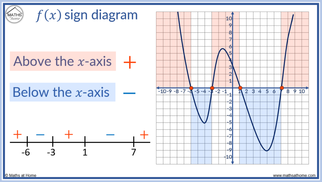
Fact

The two solutions to the quadratic equation $ax^2 + bx + c = 0$ are given by the quadratic formula:

\[ x_1, x_2 = \frac{−b \pm \sqrt{b^2 − 4ac}}{2a} \]

In other words, we have

\[ x_1 = \frac{−b + \sqrt{b^2 − 4ac}}{2a} \text{ and } x_2 = \frac{−b - \sqrt{b^2 − 4ac}}{2a} \]

Proof

The proof is by completing a square:

\[\begin{split}\begin{array}{rcl} ax^2 + bx + c &=& 0 \iff \\ x^2 + \frac{b}{a} x + \frac{c}{a} &=& 0 \iff \\ x^2 + \frac{b}{a} x &=& \frac{-c}{a} \iff \\ x^2 + \frac{2b}{2a} x &=& \frac{-c}{a} \iff \\ x^2 + 2\frac{b}{2a} x &=& \frac{-c}{a} \iff \\ x^2 + 2\frac{b}{2a} x + (\frac{b}{2a})^2 &=& \frac{-c}{a} + (\frac{b}{2a})^2 \iff \\ (x + \frac{b}{2a})(x + \frac{b}{2a}) &=& \frac{-4ac}{4a^2} + \frac{b^2}{4a^2} \iff \\ (x + \frac{b}{2a})(x + \frac{b}{2a}) &=& \frac{b^2 - 4ac}{4a^2} \iff \\ (x + \frac{b}{2a})^2 &=& \frac{b^2 - 4ac}{4a^2} \iff \\ (x + \frac{b}{2a}) &=& \pm \sqrt{\frac{b^2 - 4ac}{4a^2}} \iff \\ x &=& \frac{-b}{2a} \pm \sqrt{\frac{b^2 - 4ac}{4a^2}} \iff \\ x &=& \frac{-b}{2a} \pm \frac{\sqrt{b^2 - 4ac}}{\sqrt{4a^2}} \iff \\ x &=& \frac{-b}{2a} \pm \frac{\sqrt{b^2 - 4ac}}{2a} \iff \\ x &=& \frac{-b \pm \sqrt{b^2 - 4ac}}{2a} \\ \end{array}\end{split}\]

Definition

The discriminant of the quadratic equation $ax^2 + bx + c = 0$ is given by $D = b^2 - 4ac$.

Fact

There are three possibilities for a quadratic equation $ax^2 + bx + c = 0$:

two repeated (identical) real roots when $D = 0$
two distinct real roots when $D > 0$
no real roots (and instead two distinct complex roots) when $D < 0$

In this unit, we will not cover complex numbers. As such, we will only be interested in real solutions to quadratic equations.

Monic quadratic equation#

Consider a special case of a quadratic equation with the leading coefficient equal one, which can be obtained from a general form by dividing both sides by $a$

\[x^2 + bx + c = 0\]

The quadratic formula simplifies to

\[x_1, x_2 = \frac{−b \pm \sqrt{b^2 − 4c}}{2} = -\frac{b}{2} \pm \frac{\sqrt{b^2 − 4c}}{2} = -\frac{b}{2} \pm \sqrt{\frac{b^2}{4} − c}\]

Now observe that

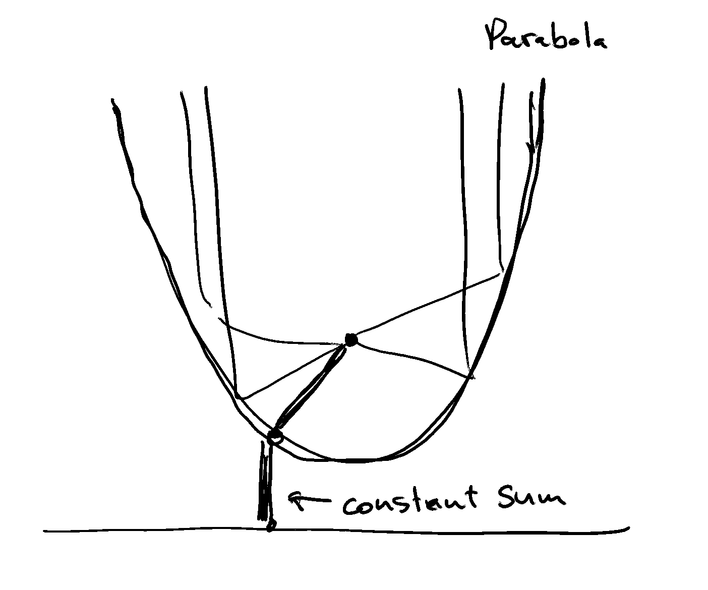
\[\left(-\frac{b}{2} + \sqrt{\frac{b^2}{4} − c}\right) + \left(-\frac{b}{2} - \sqrt{\frac{b^2}{4} − c}\right) = - \frac{b}{2}- \frac{b}{2} = -b\]

\[\left(-\frac{b}{2} + \sqrt{\frac{b^2}{4} − c}\right) \left(-\frac{b}{2} - \sqrt{\frac{b^2}{4} − c}\right) = \left(-\frac{b}{2} \right)^2 - \left(\sqrt{\frac{b^2}{4} − c}\right)^2 = c\]

Viète’s formula

The sum of the roots of a monic quadratic equation $x^2 + bx + c = 0$ is equal to $−b$ and the product of the roots is equal to $c$

\[\begin{split}x^2 + bx + c = 0 \Leftrightarrow \begin{array}{l} x_1 + x_2 = -b \\ x_1 x_2 = c \end{array} \end{split}\]

Example

\[\begin{split}\begin{array}{lcr} x^2 -3x + 2 = 0 && x_1=1, x_2=2 \\ x^2 + x -2 = 0 && x_1=1, x_2=-2 \\ x^2 + -4 = 0 && x_1=2, x_2=-2 \\ x^2 + 2x + 1 = 0 && x_1=-1, x_2=-1 \\ \end{array}\end{split}\]

The equation of a parabola#

A parabola $\mathcal{P}$ in Euclidean two-space $\mathbb{R}^2$ is a set of points with coordinates that satisfy a quadratic equation

\[\mathcal{P} = \{(x, y) \in \mathbb{R}^2: y = ax^2 + bx + c\}\]

where $a \ne 0$. The equation of this parabola is given by

\[y = ax^2 + bx + c\]

Recall the shifting of the graph mechanics to realize how the parabola shifts/compresses in space

We can complete the square to obtain the required $af(bx+c)+d$ graph-shifting form of the general quadratic function

\[ax^2 + bx + c = (\sqrt{a}x+\tfrac{b}{2\sqrt{a}})^2 + c - \tfrac{b^2}{4a} = a(x+\tfrac{b}{2a})^2 + c - \tfrac{b^2}{4a}\]

$a$ determines how tight the parabola is (squeezed/stretched across either the x or y axis)
sign of $a$ determines whether parabola is facing up or down
shifted horizontally from the origin by $\tfrac{b}{2a}$ to the left
shifted vertically by $c - \tfrac{b^2}{4a}$

Example: A quadratic break-even problem

Consider a monopolist that produces a single good. Suppose that the demand function for this good is $Q = 65 − 5P$. The monopolist has a fixed cost of $30 and a constant marginal cost of $2 per unit of the good that is produced.

The monopolist’s variable cost function is $$V (Q) = cQ$$

The monopolist’s total cost function is

\[\begin{split} \begin{align*} C(Q) &= F + V(Q) \\ &= F + cQ \\ &= 30 + 2Q \end{align*} \end{split}\]

Let the given inverse demand function be

\[ P^D = 13 − \frac{1}{5} Q\]

The monopolist’s total revenue function is then given by

\[\begin{split} \begin{align*} R(Q) &= P^D (Q) Q \\ &= (13 − \frac{1}{5}Q) Q \\ &= 13Q − \frac{1}{5} Q^2 \end{align*} \end{split}\]

The monopolist’s profit function is

\[\begin{split} \begin{align*} \pi(Q) &= R(Q) − C(Q) \\ &= 13Q − \frac{1}{5} Q^2 − (30 + 2Q) \\ &= 13Q − \frac{1}{5} Q^2 − 30 - 2Q \\ &= −\frac{1}{5} Q^2 + 11Q − 30 \\ \end{align*} \end{split}\]

Note that this monopolist’s profit function is an “upside down” parabola

The firm will break-even when it makes exactly zero profit. This requires that $\pi(Q) = 0$, which in turn requires that

\[ −\frac{1}{5} Q^2 + 11Q − 30 = 0 \]

Upon multiplying both sides of this quadratic equation by (−5), we obtain another quadratic equation of the form

\[ Q^2 - 55Q + 150 = 0 \]

This second quadratic equation is equivalent to the first quadratic equation in the sense that it will have identical solution values for the variable $Q$

We know from the quadratic formula that

\[\begin{split} \begin{align*} Q_1, Q_2 &= \frac{−(−55) \pm \sqrt{(−55)^2 − 4(150)}}{2} \\ &= \frac{55 \pm \sqrt{3025 − 600}}{2} \\ &= \frac{55 \pm \sqrt{2425}}{2} \\ &\approx \frac{55 \pm 49.24}{2} \\ &\approx \frac{104.24}{2} \frac{5.76}{2} \\ &\approx 52.12, 2.88 \end{align*} \end{split}\]

Thus the monopolist will make:

negative profits when $Q \in (0, 2.88) \cup (52.12, \infty)$ (approximately),
zero profits when $Q \in \{2.88, 52.12\}$ (approximately), and
positive profits when $Q \in (2.88, 52.12)$ (approximately)

The break-even points are $Q \approx 2.88$ units of output and $Q \approx 52.12$ units of output.

[Bradley, 2013] Example 4.9 on pp. 162-163

Higher order polynomial equations#

We have seen that polynomial equations with $n \in \{1,2\}$ have nice formulas for their solutions.

“Nice” is dependent on the coefficients, involving algebra and radicals (square and possibly $n$-roots)

What happens in higher orders?

$n = 3$#

Consider the following polynomial of degree three:

\[f(x) = ax^3 + bx^2 + cx + d\]

where $a \ne 0$. This is a cubic function. The corresponding polynomial equation is a cubic equation.

\[ax^3 + bx^2 + cx + d = 0, \; a \ne 0\]

Solving the cubic equation has a rich history (see excellent videos linked in the end of this note).

The formulas known today are known as Cardano’s formulas, and they are quite complex 🤓

\[p = \frac{3ac - b^2}{3a^2} \text{ and } q = \frac{2b^3 - 9abc + 27a^2d}{27a^3}\]

\[x = \sqrt[3]{-\frac{q}{2} + \sqrt{\frac{q^2}{4} + \frac{p^3}{27}}} + \sqrt[3]{-\frac{q}{2} - \sqrt{\frac{q^2}{4} + \frac{p^3}{27}}}\]

The substitutions are due to the substitution $x \rightarrow x-\tfrac{b}{3a}$. We get

\[\begin{split}\begin{array}{l} \big(x-\tfrac{b}{3a}\big)^3 + \tfrac{b}{a}\big(x-\tfrac{b}{3a}\big)^2 + \tfrac{c}{a}\big(x-\tfrac{b}{3a}\big) + \tfrac{d}{a} = 0 \\ x^3 + x^2 \big[ \tfrac{b}{a} - \tfrac{b}{a}\big] + x \big[ \tfrac{c}{a} - \tfrac{b^2}{3a}\big] + \tfrac{2b^3}{27a^3} - \tfrac{bc}{3a^2} + \tfrac{d}{a} = 0 \end{array}\end{split}\]

\[x^3 + px + q = 0\]

Definition

This form of cubic equation is called depressed cubic.

Example

\[x^3 - 15x - 126 = 0\]

\[\begin{split}x =& \sqrt[3]{63 + \sqrt{63^2 - 5^3}} + \sqrt[3]{63 - \sqrt{63^2 - 5^3}} =\\ =& \sqrt[3]{63 + \sqrt{3844}} + \sqrt[3]{63 - \sqrt{3844}}=\\ =& \sqrt[3]{63 + 62} + \sqrt[3]{63 - 62}=\\ =& \sqrt[3]{125} + \sqrt[3]{1}=\\ =& 5 + 1 = 6\end{split}\]

Source: Mathologer

Example

\[x^3 - 6x - 40 = 0\]

\[\begin{split}x =& \sqrt[3]{20 + \sqrt{20^2 - 2^3}} + \sqrt[3]{20 - \sqrt{20^2 - 2^3}} =\\ =& \sqrt[3]{20 + \sqrt{392}} + \sqrt[3]{20 - \sqrt{392}}=\\ =& \sqrt[3]{20 + 14\sqrt{2}} + \sqrt[3]{20 - 14\sqrt{2}}\end{split}\]

But for $x=4$ we have $64 - 24 -40 = 0$, so $x=4$ is a solution to the equation!

\[4 = \sqrt[3]{20 + 14\sqrt{2}} + \sqrt[3]{20 - 14\sqrt{2}} \quad\text{???}\]

Source: Mathologer

Example

\[x^3 - 6x - 4 = 0\]

\[\begin{split}x =& \sqrt[3]{2 + \sqrt{2^2 - 2^3}} + \sqrt[3]{2 - \sqrt{2^2 - 2^3}} =\\ =& \sqrt[3]{2 + \sqrt{-4}} + \sqrt[3]{2 - \sqrt{-4}}\end{split}\]

However, we can check by plugging the values back into the equation that $x_1=-2$, $x_2=1-\sqrt{3}$ are $x_3=1+\sqrt{3}$ are the three real solutions to the equation!

Source and further explanation: Mathologer

Example (preview into the complex numbers)

Let’s look at the simplest case

\[x^3 = 1\]

Solution is $x = 1$. But where are the other two solutions?

Well, remember that $x^3-1 = (x-1)(x^2+x+1)$ $\Rightarrow$ the other two roots must be in the quadratic equation.

Applying the quadratic formula and denoting $\sqrt{-1}=i \Leftrightarrow i^2=-1$ we have

\[x = \frac{-1 \pm \sqrt{1^2 - 4}}{2} = \frac{-1 \pm \sqrt{-3}}{2} = \frac{-1 \pm i\sqrt{3}}{2}\]

Let’s verify that these are indeed the solutions to $x^3 = 1$

\[\begin{split}\begin{array}{l} \left( \frac{-1 + i\sqrt{3}}{2} \right)^2 = \frac{1}{4} \big[ (-1)^2 + 2(-1)i\sqrt{3} + (i\sqrt{3})^2 \big] = \\ = \frac{1}{4} \big[ 1 - 2i\sqrt{3} + 3(i)^2 \big] = \frac{1}{4} \big[ 1 - 2i\sqrt{3} - 3 \big] = \frac{-1 - i\sqrt{3}}{2} \\ \left( \frac{-1 + i\sqrt{3}}{2} \right)^3 = \frac{(-1 - i\sqrt{3})}{2} \frac{(-1 + i\sqrt{3})}{2} = \\ = \frac{1}{4}\big[ (-1)^2 - (i\sqrt{3})^2 \big] = \frac{1-3i^2}{4} = \frac{1+3}{4} = 1 \\ \left( \frac{-1 - i\sqrt{3}}{2} \right)^2 = \frac{1}{4} \big[ (-1)^2 - 2(-1)i\sqrt{3} + (i\sqrt{3})^2 \big] = \\ = \frac{1}{4} \big[ 1 + 2i\sqrt{3} + 3(i)^2 \big] = \frac{1}{4} \big[ 1 + 2i\sqrt{3} - 3 \big] = \frac{-1 + i\sqrt{3}}{2}\\ \left( \frac{-1 - i\sqrt{3}}{2} \right)^3 = \frac{(-1 + i\sqrt{3})}{2} \frac{(-1 - i\sqrt{3})}{2} = 1 \end{array}\end{split}\]

Therefore, all of the solution of $x^3=1$ are $x_1=1$, $x_2=\frac{(-1 + i\sqrt{3})}{2}$ and $x_3=\frac{(-1 - i\sqrt{3})}{2}$, where $x_1 \in \mathbb{R}$ and $x_2,x_3 \in \mathbb{C}$ (complex numbers).

_images/cube-root-root-of-unity.png — Fig. 22 Cubic roots of unity#

there are exactly $n$ complex roots to the equation $x^n=1$ according to the Fundamental theorem of algebra
these roots are evenly distributed along the unit circle in the complex plane
taking a power $n$ of each root rotates the point along the unit circle
therefore any root of unity to power $n$ lands exactly at 1

Definition

Roots of unity are complex solutions to an equation $x^n=1$

radicals such as $\sqrt[3]{\cdot}$ applied to complex numbers result in multiple points!
the Cardano’s formulas operate in the complex plain
therefore even when the solutions to a cubic equation are real, the expressions may involve complex numbers!

$n = 4$#

We concluded that already for $n=3$ it is impossible to avoid complex plain in the formulas for the solutions

Consider the following polynomial of degree three:

\[f(x) = ax^4 + bx^3 + cx^2 + dx + e\]

where $a \ne 0$. This is a quartic function. The corresponding polynomial equation is a quartic equation.

\[ax^3 + bx^2 + cx + d = 0, \; a \ne 0\]

Solutions of the quartic equation can be written by formulas involving polynomial coefficients and radicals (Ferrari formulas), but they become practically unusable

$n \geqslant 5$#

Fact (Abel’s theorem)

For $n>4$ the roots of the polynomial equation

\[x^n + b_{n − 1} x^{n − 1} + · · · + b_1 x + b_0 = 0\]

can not be expressed in terms of radicals.

Proof involves high level abstract math (Galois theory)

Case closed!

Factorization of polynomials#

When we have to solve a higher order polynomial equation, we can go back to the Fundamental theorem of algebra and try make a few steps on the way to represent the polynomial as a product of linear factors

\[\begin{split}\begin{align*} f(x) &= x^n + b_{n − 1} x^{n − 1} + · · · + b_1 x + b_0 \\ &= (x − x_1) (x − x_2) · · · (x − x_n) \\ &= \prod_{k = 1}^{n} (x − x_k) \end{align*}\end{split}\]

Fact

Polynomial equation in the form

\[\prod_{k = 1}^{n} (x − x_k) =0\]

has exacly $n$ solutions $\{x_1,\dots,x_n\}$.

Fact

The set of solutions of the polynomial equation in the form

\[(x^n + a_{n − 1} x^{n − 1} + · · · + a_1 x + a_0)(x^m + b_{m − 1} x^{m − 1} + · · · + b_1 x + b_0)=0\]

is a union of the roots of the two polynomials.

Therefor, through factorization of the polynomials, we may be able to find some if not all solutions.

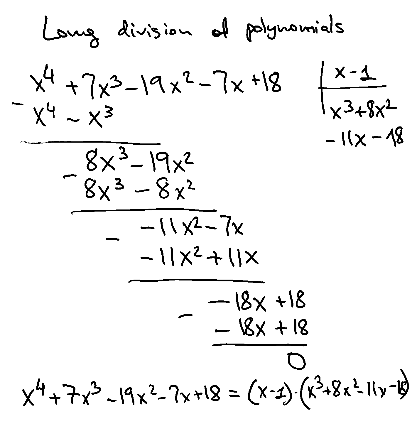
Example

\[x^4 +7x^3−19x^2−7x+18 = 0\]

We may notice that $x^4 +7x^3−19x^2−7x+18 = (x-1)(x^3+8x^2-11x-18)$, giving $x=1$ as one of four of the solutions

We can use long division to factorize the higher order polynomial into a product of lower order polynomials

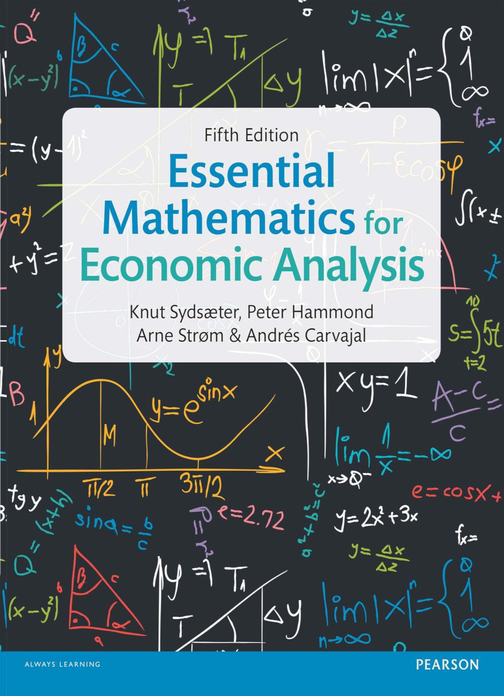
Example

Consider the rational function $R(x) = \frac{x^2 + x − 1}{x − 1}$. Note the following.

Thus we have

\[ R(x) = \frac{x^2 + x − 1}{x − 1} = (x + 2) + \left( \frac{1}{x − 1} \right) \]

try to factor out simple binomials like $x-1$, $x+1$ and so on
remembering some standard formulas will be very helpful

\[\begin{split}\begin{array}{c} a^2 - b^2 = (a + b)(a - b) \\ (a + b)^2 = a^2 + 2ab + b^2 \\ (a + b)^3 = a^3 + 3a^2b + 3ab^2 + b^3 \\ (a - b)^3 = a^3 - 3a^2b + 3ab^2 - b^3 \\ a^3 + b^3 = (a + b)(a^2 - ab + b^2) \\ a^3 - b^3 = (a - b)(a^2 + ab + b^2) \end{array}\end{split}\]

but generally very tedious and time consuming process

Example

\[x^5 - x^4 -15 x^3 -23x^2 -26x -24 =0\]

Follow on the board

Hint: $x-1$, $x+1$, $x-2$, $x-3$, $x+4$

Inequalities#

General algorithm:

to solve an inequality $h(x)\geqslant0$ we need to find the set of values for which $h(x)=0$ to determine the points where $h(x)$ changes its sign 2.once these points are found by solving $h(x)=0$, we can to determine the signs of $h(x)$ in the intervals between these points.

Much of the above theory applies!

Elementary inequality transformations#

Fact

For $a,b,c,d \in \mathbb{R}$

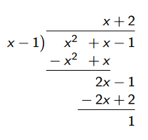
\[\begin{split}\begin{array}{r} a>b \text{ and } b>c \Rightarrow a>c \\ a>b \text{ and } c>0 \Rightarrow ac > bc \\ a>b \text{ and } c<0 \Rightarrow ac < bc \\ a>b \text{ and } c>d \Rightarrow a+c > b+d \\ a>b \text{ and } f(x) \text{ is monotonically increasing} \Rightarrow f(a) > f(b) \\ a>b \text{ and } g(x) \text{ is monotonically decreasing} \Rightarrow g(a) < g(b) \end{array}\end{split}\]

Sign diagrams#

Fact

For a polynomial $h(x) = a_n x^n + a_{n − 1} x^{n − 1} + · · · + a_1 x + a_0$, $a_n \ne 0$ with distinct roots $\{x_1,\dots,x_n\}$, which break up the number line into $n+1$ intervals, the sign of $h(x)$ alternates on these intervals.

Example

\[(x+1)(x-2)<=0\]

The roots are $x_1=-1$ and $x_2=2$. There are three intervals $(-\infty,-1)$, $(-1,2)$ and $(2,\infty)$. The sign of the polynomial changes on each of these intervals

Interval	$x+1$	$x-2$	$h(x)$
$(-\infty,-1)$	$-$	$-$	$+$
$(-1,2)$	$+$	$-$	$-$
$(2,\infty)$	$+$	$+$	$+$

Therefore the solution to the inequality is $x \in [-1,2]$. Note that the interval is closed because the inequality is non-strict

Example

\[\frac{2x-3}{x-1} \leqslant 3-x\]

Wrong! Multiply both sides by $(x-1)$ to simplify. This can not be done unless we know the sign of $(x-1)$

Instead rewrite as

\[\frac{2x-3 + (x-1)(x-3)}{x-1} \leqslant 0 \]

The enumerator can be simplified to $x^2-2x = x(x-2)$, leading to the following sign diagram

Interval	$x$	$x-1$	$x-2$	$h(x)$
$(-\infty,0)$	$-$	$-$	$-$	$-$
$(0,1)$	$+$	$-$	$-$	$+$
$(1,2)$	$+$	$+$	$-$	$-$
$(2,\infty)$	$+$	$+$	$+$	$+$

Note! It is very important to remember that $x=1$ is not in the domain of the RHS, therefore should not appear in the solution!

The solution is $(-\infty,0] \cup (1,2]$

Double inequalities and inequalities with absolute value#

Definition

A double inequality of the form

\[a \leqslant h(x) \leqslant b\]

is equivalent to two inequalities holding simultaneously

\[\begin{split}\begin{cases} h(x) \geqslant a \\ h(x) \leqslant b \end{cases}\end{split}\]

To solve a double inequality:

solve the two inequalities separately
take the intersection of the two solution sets

Fact

For any function $h(x):\mathbb{R} \to \mathbb{R}$ an inequality of the form

\[|h(x)| \leqslant a\]

is equivalent to the double inequality

\[-a \leqslant h(x) \leqslant a\]

Example

\[|x - 3| < 2\]

This is equivalent to

\[\begin{split}\begin{cases} x-3 < 2 \\ x-3 > -2 \end{cases}\end{split}\]

Solving the first inequality we have $x<5$ and solving the second we have $x>1$. Therefore the solution is $(1,5)$.

Notes from the lecture#

Hand written notes from the lecture

Interval	\(x+1\)	\(x-2\)	\(h(x)\)
\((-\infty,-1)\)	\(-\)	\(-\)	\(+\)
\((-1,2)\)	\(+\)	\(-\)	\(-\)
\((2,\infty)\)	\(+\)	\(+\)	\(+\)

Interval	\(x\)	\(x-1\)	\(x-2\)	\(h(x)\)
\((-\infty,0)\)	\(-\)	\(-\)	\(-\)	\(-\)
\((0,1)\)	\(+\)	\(-\)	\(-\)	\(+\)
\((1,2)\)	\(+\)	\(+\)	\(-\)	\(-\)
\((2,\infty)\)	\(+\)	\(+\)	\(+\)	\(+\)

📖 Equations and inequalities

Contents

📖 Equations and inequalities#

General equations/inequalities#

Elementary transformations#

Solving equations and inequalities#

Polynomial equations#

Solutions of polynomial equations#

Linear equations#

The equation of a straight line#

Point-slope formula#

Two-point formula#

Rise over run#

X and Y intercepts of a straight line#

Quadratic equations#

Monic quadratic equation#

The equation of a parabola#

Higher order polynomial equations#

\(n = 3\)#

\(n = 4\)#

\(n \geqslant 5\)#

Factorization of polynomials#

Inequalities#

Elementary inequality transformations#

Sign diagrams#

Double inequalities and inequalities with absolute value#

Notes from the lecture#