📖 Systems of linear equations

📖 Systems of linear equations#

⏱ | words

What is a system of linear equations#

Definition

A general system of linear equations can be written as

\[\begin{split} \begin{array}{c} a_{11} x_1 + a_{12} x_2 + \cdots + a_{1K} x_K = b_1 \\ a_{21} x_1 + a_{22} x_2 + \cdots + a_{2K} x_K = b_2 \\ \vdots \\ a_{N1} x_1 + a_{N2} x_2 + \cdots + a_{NK} x_K = b_N \end{array} \end{split}\]

More often we write the system in matrix form

\[\begin{split} \left( \begin{array}{cccc} a_{11} & a_{12} & \cdots & a_{1K} \\ a_{21} & a_{22} & \cdots & a_{2K} \\ \vdots & \vdots & & \vdots \\ a_{N1} & a_{N2} & \cdots & a_{NK} \end{array} \right) \left( \begin{array}{c} x_1 \\ x_2 \\ \vdots \\ x_K \end{array} \right) = \left( \begin{array}{c} b_1 \\ b_2 \\ \vdots \\ b_K \end{array} \right) % \end{split}\]

\[ % A x = b % \]

A solution to the system of equations is a vector \(x\) that satisfies \(Ax=b\).

To solve the system of equation, similar to solving an equation, is to find all elements of the set of the solutions, or establish that this set is empty.

Gaussian elimination#

Gaussian elimination is a simple manual algorithm for solving linear systems

Think long division: you can do solve it using computer or calculator, but handy to be able to do it by hand too

Definition

Augmented matrix notation for the system of linear equations has an extra column made by the RHS of the system:

\[\begin{split} \left( \begin{array}{cccc|c} a_{11} & a_{12} & \cdots & a_{1K} & b_1 \\ a_{21} & a_{22} & \cdots & a_{2K} & b_2 \\ \vdots & \vdots & & \vdots & \vdots \\ a_{N1} & a_{N2} & \cdots & a_{NK} & b_K \end{array} \right) \end{split}\]

Gaussian elimination is a method for solving systems of linear equations which consists of performing operations on the rows of the augmented matrix that represents the system.
The goal is to transform this matrix into an upper triangular or row-echelon form
From there, solutions can be easily obtained through back substitution

Definition: Elementary row operations

Let \(R_i\) denote a row of the augmented matrix of the system

Swap two rows \(R_i \leftrightarrow R_j\)
Multiply a row by a nonzero scalar \(C \cdot R_i \rightarrow R_i\), \(C>0\)
Add a multiple of one row to another row \(kR_i + R_j \rightarrow R_j\)

Example

Let’s solve the following system of linear equations:

\[\begin{split} \begin{align*} x + 2y + z &= 5, \\ 3x + 3y + 6z &= 15, \\ 2x + 4y + 4z &= 12. \end{align*} \end{split}\]

The augmented matrix corresponding to the system is:

\[\begin{split} \left( \begin{array}{ccc|c} 1 & 2 & 1 & 5 \\ 3 & 3 & 6 & 15 \\ 2 & 4 & 4 & 12 \end{array} \right) \rightarrow \end{split}\]

Perform elementary row operations. Goal: Form an upper triangular matrix.

Step 1: Eliminate \(x\) from the second row \(R_2 - 3R_1 \rightarrow R_2\)

\[\begin{split} \left( \begin{array}{ccc|c} 1 & 2 & 1 & 5 \\ 0 & -3 & 3 & 0 \\ 2 & 4 & 4 & 12 \end{array} \right) \rightarrow \end{split}\]

Step 2: Eliminate \(x\) from the third rows \(R_3 - 2R_1 \rightarrow R_3\)

\[\begin{split} \left( \begin{array}{ccc|c} 1 & 2 & 1 & 5 \\ 0 & -3 & 3 & 0 \\ 0 & 0 & 2 & 2 \end{array} \right) \rightarrow \end{split}\]

Step 3: Make the pivot in the second row \(-\frac{1}{3}R_2 \rightarrow R_2\)

\[\begin{split} \left( \begin{array}{ccc|c} 1 & 2 & 1 & 5 \\ 0 & 1 & -1 & 0 \\ 0 & 0 & 2 & 2 \end{array} \right) \rightarrow \end{split}\]

Step 4: Make the pivot in the third row \(\frac{1}{2}R_3 \rightarrow R_3\)

\[\begin{split} \left( \begin{array}{ccc|c} 1 & 2 & 1 & 5 \\ 0 & 1 & -1 & 0 \\ 0 & 0 & 1 & 1 \end{array} \right) \end{split}\]

(\(\star\)) Now we have a triangular matrix, and we can perform back substitution to find the values of \(z\), \(y\), and \(x\) in return.

\[\begin{split} \begin{array}{l} z = 1 \\ y - 1 = 0 \quad \Rightarrow \quad y = 1 \\ x + 2 + 1 = 5 \quad \Rightarrow \quad x = 2 \end{array} \end{split}\]

The solution is \((x,y,z) = (2,1,1)\)

We could continue elementary row operations after (\(\star\)) to get the identity matrix in the first block. These steps are referred to as Gauss-Jordan elimination steps

\[\begin{split} \left( \begin{array}{ccc|c} 1 & 2 & 1 & 5 \\ 0 & 1 & -1 & 0 \\ 0 & 0 & 1 & 1 \end{array} \right) \rightarrow \end{split}\]

Step 5: Eliminate \(z\) in the second row \(R_2 + R_3 \rightarrow R_2\)

\[\begin{split} \left( \begin{array}{ccc|c} 1 & 2 & 1 & 5 \\ 0 & 1 & 0 & 1 \\ 0 & 0 & 1 & 1 \end{array} \right) \rightarrow \end{split}\]

Step 6: Eliminate \(z\) in the first row \(R_1 - R_3 \rightarrow R_1\)

\[\begin{split} \left( \begin{array}{ccc|c} 1 & 2 & 0 & 4 \\ 0 & 1 & 0 & 1 \\ 0 & 0 & 1 & 1 \end{array} \right) \rightarrow \end{split}\]

Step 6: Eliminate \(y\) in the first row \(R_1 - 2 R_2 \rightarrow R_1\)

\[\begin{split} \left( \begin{array}{ccc|c} 1 & 0 & 0 & 2 \\ 0 & 1 & 0 & 1 \\ 0 & 0 & 1 & 1 \end{array} \right) \end{split}\]

At this stage the system is trivial, each equation contains a single variable with 1 as a coefficient. We can just read out the solution \((x,y,z) = (2,1,1)\)

Definition

A matrix is said to be in row echelon form if it satisfies the following conditions:

all rows having only zero entries are at the bottom of the matrix
leading entry (first non-zero entry) of each row is to the right of the leading entry of the row above it

A matrix is said to be in reduced row echelon form if it satisfies one additional condition:

the leading entry in each row is 1
each column containing a leading 1 has all other entries equal to zero

The first nonzero entry of each row is called a pivot

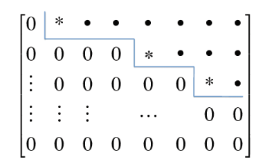
_images/row_echelon.png — Fig. 31 Structure of row echelon matrix#

Gaussian elimination leads to the row echelon form of the matrix
Gaussian-Jordan elimination leads to the reduced row echelon form of the matrix

Fact

Every matrix has a unique reduced row echelon form.

Fact

Every matrix can be transformed to echelon and reduced echelon form using Gaussian elimination.

The difference between row echelon and upper-triangular:

upper-triangular: all entries below the diagonal are zero, square matrix (right)
row echelon: defined for any shape, zero rows must be on the bottom (left)

\[\begin{split} \begin{pmatrix} 1 & 2 & 3 & 4 \\ 0 & 1 & 4 & 0 \\ 0 & 0 & 0 & 2 \end{pmatrix} \quad\quad \begin{pmatrix} 1 & 2 & 3 \\ 0 & 0 & 0 \\ 0 & 0 & 7 \end{pmatrix} \end{split}\]

System with no solutions#

Example

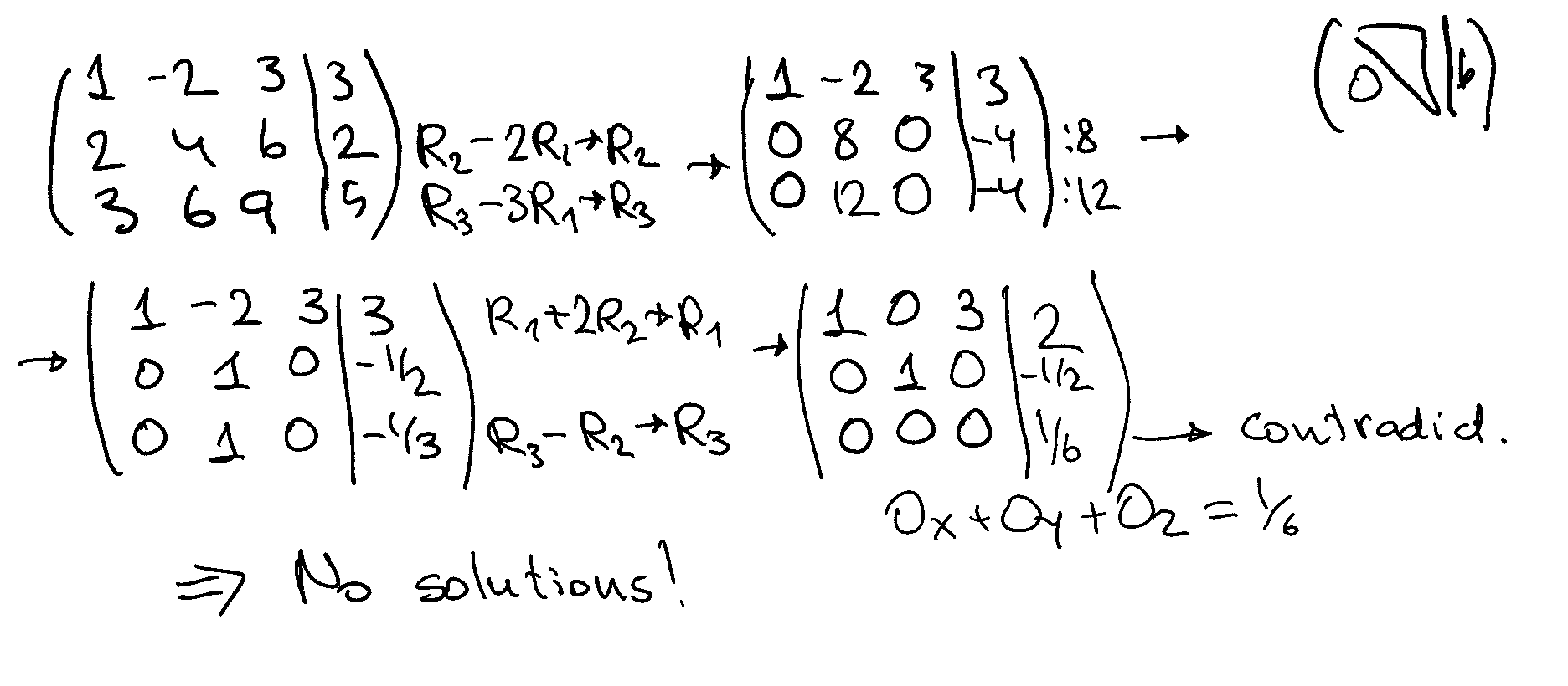
\[\begin{split} \begin{align*} x - 2y + 3z &= 3, \\ 2x + 4y + 6z &= 2, \\ 3x + 6y + 9z &= 5. \end{align*} \end{split}\]

\[\begin{split} \begin{array}{ll} \left(\begin{array}{ccc|c} 1 & -2 & 3 & 3 \\ 2 & 4 & 6 & 2 \\ 3 & 6 & 9 & 5 \end{array}\right) \begin{array}{l} \\ R_2 - 2 R_1 \to R_2 \\ R_3 - 3 R_1 \to R_3 \\ \end{array} &\longrightarrow \end{array} \end{split}\]

\[\begin{split} \begin{array}{ll} \left(\begin{array}{ccc|c} 1 & -2 & 3 & 3 \\ 0 & 8 & 0 & -4 \\ 0 & 12 & 0 & -4 \end{array}\right) \begin{array}{l} \\ R_2/8 \to R_2 \\ R_3 /12 \to R_3 \\ \end{array} &\longrightarrow \end{array} \end{split}\]

\[\begin{split} \begin{array}{ll} \left(\begin{array}{ccc|c} 1 & -2 & 3 & 3 \\ 0 & 1 & 0 & -1/2 \\ 0 & 1 & 0 & -1/3 \end{array}\right) \begin{array}{l} R_1+2R_2 \to R_2\\ R_3-R_2 \to R_3\\ \\ \end{array} &\longrightarrow \end{array} \end{split}\]

\[\begin{split} \left(\begin{array}{ccc|c} 1 & 0 & 3 & 2 \\ 0 & 1 & 0 & -1/2 \\ 0 & 0 & 0 & 1/6 \end{array}\right) \end{split}\]

The last row corresponds to the equation \(0 = 1/6\), which is a contradiction. Therefore, the system has no solutions.

Fact

If the last row of the row-echelon form of the augmented matrix corresponds to the equation \(0 = c\), where \(c \neq 0\), then the system of linear equations has no solutions.

System with non-unique solutions#

Example: no unique solution

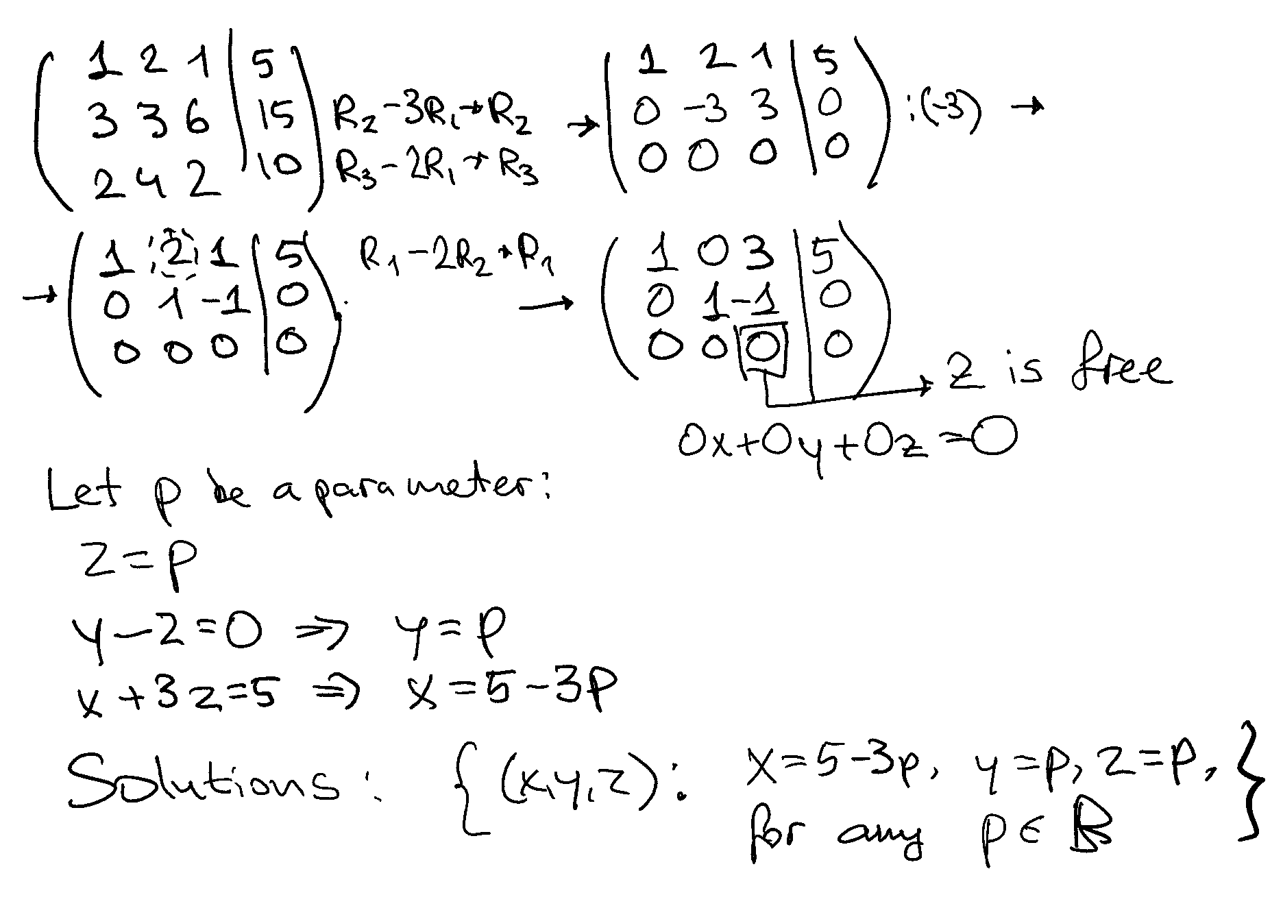
\[\begin{split} \begin{align*} x + 2y + z &= 5, \\ 3x + 3y + 6z &= 15, \\ 2x + 4y + 2z &= 10. \end{align*} \end{split}\]

\[\begin{split} \begin{array}{ll} \left(\begin{array}{ccc|c} 1 & 2 & 1 & 5 \\ 3 & 3 & 6 & 15 \\ 2 & 4 & 2 & 10 \end{array}\right) \begin{array}{l} \\ R_2 - 3 R_1 \to R_2 \\ R_3 - 2 R_1 \to R_3 \\ \end{array} &\longrightarrow \end{array} \end{split}\]

\[\begin{split} \begin{array}{ll} \left(\begin{array}{ccc|c} 1 & 2 & 1 & 5 \\ 0 & -3 & 3 & 0 \\ 0 & 0 & 0 & 0 \end{array}\right) \begin{array}{l} \\ -\tfrac{1}{3} R_2 \to R_2 \\ \\ \end{array} &\longrightarrow \end{array} \end{split}\]

\[\begin{split} \begin{array}{ll} \left(\begin{array}{ccc|c} 1 & 2 & 1 & 5 \\ 0 & 1 & -1 & 0 \\ 0 & 0 & 0 & 0 \end{array}\right) \begin{array}{l} R_1 - 2 R_2 \to R_1\\ \\ \\ \end{array} &\longrightarrow \end{array} \end{split}\]

\[\begin{split} \left(\begin{array}{ccc|c} 1 & 0 & 3 & 5 \\ 0 & 1 & -1 & 0 \\ 0 & 0 & 0 & 0 \end{array}\right) \end{split}\]

Note that the last row with all zero places no restriction on \(z\) which we can let equal to parameter \(t\), \(z = t\).

from \(R_2\): \(y = t\)
from \(R_1\): \(x = 5 - 3 t\)

Thus, the solution in parametric form:

\[\begin{split} \begin{align*} x &= 5 - 3t, \\ y &= t, \\ z &= t, \end{align*} \end{split}\]

where \(t\) is a parameter.

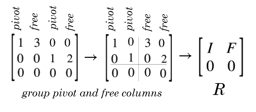
_images/echelon_pivot_free.png — Fig. 32 Systems with free variables#

Fact

The variables corresponding to the columns without a pivot in the row-echelon form of the augmented matrix referred to as free variables play the role of parameters in the non-unique solution of the system of linear equations.

Inverse by Gaussian row operations#

In order to find the inverse of the \(P\) matrix, we make the following argument. By definition, \(PP^{-1} = I\), and therefore the columns of the unknown matrix \(P^{-1}\) (denoted below \(p'_i\), \(i=1,2,3\)) are solutions of the following three systems of equations:

\[\begin{split} P p'_1 = \begin{pmatrix} 1 \\ 0 \\ 0 \end{pmatrix} \quad P p'_2 = \begin{pmatrix} 0 \\ 1 \\ 0 \end{pmatrix} \quad P p'_3 = \begin{pmatrix} 0 \\ 0 \\ 1 \end{pmatrix} \end{split}\]

We can find the solutions of all three systems by Gaussian elimination performing elementary row operations on an ``extra’’ augmented matrix with three columns in place of the right-hand side.

Example

Let’s find the inverse of the matrix

\[\begin{split} P = \left(\begin{array}{ccc} 0 & 2/\sqrt{5} & 1/\sqrt{2} \\ 0 & 1/\sqrt{5} & -1/\sqrt{2} \\ 1 & 0 & 0 \end{array}\right) \end{split}\]

\[\begin{split} \left(\begin{array}{ccc|ccc} 0 & 2/\sqrt{5} & 1/\sqrt{2} & 1 & 0 & 0 \\ 0 & 1/\sqrt{5} & -1/\sqrt{2} & 0 & 1 & 0 \\ 1 & 0 & 0 & 0 & 0 & 1 \end{array}\right) \longrightarrow \end{split}\]

\[\begin{split} \left(\begin{array}{ccc|ccc} 1 & 0 & 0 & 0 & 0 & 1 \\ 0 & 1 & -\sqrt{5}/\sqrt{2} & 0 & \sqrt{5} & 0 \\ 0 & 2/\sqrt{5} & 1/\sqrt{2} & 1 & 0 & 0 \end{array}\right) \longrightarrow \end{split}\]

\[ \frac{1}{\sqrt{2}} + \left(-\frac{\sqrt{5}}{\sqrt{2}}\right)\left(-\frac{2}{\sqrt{5}}\right) = \frac{1}{\sqrt{2}} + \frac{2}{\sqrt{2}} = \frac{3}{\sqrt{2}} \]

\[\begin{split} \left(\begin{array}{ccc|ccc} 1 & 0 & 0 & 0 & 0 & 1 \\ 0 & 1 & -\sqrt{5}/\sqrt{2} & 0 & \sqrt{5} & 0 \\ 0 & 0 & 3/\sqrt{2} & 1 & -2 & 0 \end{array}\right) \longrightarrow \end{split}\]

\[\begin{split} \left(\begin{array}{ccc|ccc} 1 & 0 & 0 & 0 & 0 & 1 \\ 0 & 1 & -\sqrt{5}/\sqrt{2} & 0 & \sqrt{5} & 0 \\ 0 & 0 & 1 & \sqrt{2}/3 & -2\sqrt{2}/3 & 0 \end{array}\right) \longrightarrow \end{split}\]

\[ \sqrt{5} + \frac{\sqrt{5}}{\sqrt{2}} \left(-\frac{2 \sqrt{2}}{3} \right) = \frac{\sqrt{5}}{3} \]

\[\begin{split} \left(\begin{array}{ccc|ccc} 1 & 0 & 0 & 0 & 0 & 1 \\ 0 & 1 & 0 & \sqrt{5}/3 & \sqrt{5}/3 & 0 \\ 0 & 0 & 1 & \sqrt{2}/3 & -2\sqrt{2}/3 & 0 \end{array}\right) \longrightarrow \end{split}\]

Therefore, the inverse of the \(P\) matrix is given by

\[\begin{split} P^{-1} = \begin{pmatrix} 0 & 0 & 1 \\ \sqrt{5}/3 & \sqrt{5}/3 & 0 \\ \sqrt{2}/3 & -2\sqrt{2}/3 & 0 \end{pmatrix} \end{split}\]

Solving a linear system using matrix inverse#

Assuming that the matrix \(A\) is invertible, the solution to the system of linear equations \(Ax=b\) can be found by multiplying both sides by the inverse of \(A\):

\[\begin{split} \begin{array}{rcl} Ax &=& b \\ A^{-1}Ax &=& A^{-1}b \\ x &=& A^{-1}b \end{array} \end{split}\]

Example

\[\begin{split} \left(\begin{array}{ccc} 0 & 2/\sqrt{5} & 1/\sqrt{2} \\ 0 & 1/\sqrt{5} & -1/\sqrt{2} \\ 1 & 0 & 0 \end{array}\right) \begin{pmatrix} x \\ y \\ z \end{pmatrix} = \begin{pmatrix} 3 \\ 3 \\ 2 \end{pmatrix} \end{split}\]

\[\begin{split} \begin{pmatrix} x \\ y \\ z \end{pmatrix} = \begin{pmatrix} 0 & 0 & 1 \\ \sqrt{5}/3 & \sqrt{5}/3 & 0 \\ \sqrt{2}/3 & -2\sqrt{2}/3 & 0 \end{pmatrix} \begin{pmatrix} 3 \\ 3 \\ 2 \end{pmatrix} = \begin{pmatrix} 2 \\ 2\sqrt{5} \\ -\sqrt{2} \end{pmatrix} \end{split}\]

Determinants under Gaussian elimination#

Fact

Elementary operations on the rows of a square matrix have the following effect on its determinant:

Swap two rows \(R_i \leftrightarrow R_j\) \(\Longrightarrow\) Determinant changes sign
Multiply a row by a nonzero scalar \(C \cdot R_i \rightarrow R_i\), \(C>0\) \(\Longrightarrow\) Determinant is multiplied by the same scalar \(C\)
Add a multiple of one row to another row \(kR_i + R_j \rightarrow R_j\) \(\Longrightarrow\) Determinant does not change!

Example

\[\begin{split} \det \begin{pmatrix} 1 & 1 & 1 \\ x & y & z \\ x^2 & y^2 & z^2 \end{pmatrix} = \det \begin{pmatrix} 1 & 0 & 0 \\ x & y-x & z-x \\ x^2 & y^2-x^2 & z^2-x^2 \end{pmatrix} = \end{split}\]

\[\begin{split} = \det \begin{pmatrix} y-x & z-x \\ y^2-x^2 & z^2-x^2 \end{pmatrix} = \end{split}\]

\[\begin{split} = (y-x)(z-x) \det \begin{pmatrix} 1 & 1 \\ x+y & x+z \end{pmatrix} = \end{split}\]

\[ = (y-x)(z-x)(x+z-x-y)=(y-x)(z-x)(z-y) \]

Inverse by determinants#

Recall from the previous lecture

Definition

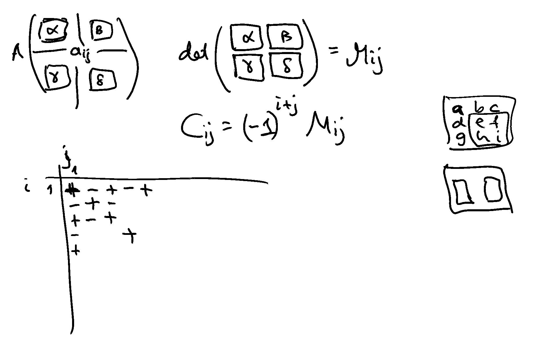
Consider an \(n \times n\) matrix \(A\). Denote \(A_{ij}\) a \((n-1) \times (n-1)\) submatrix of \(A\), obtained by deleting the \(i\)-th row and \(j\)-th column of \(A\). Then

the \((i,j)\)-th minor of \(A\) denoted \(M_{ij}\) is

\[ M_{ij} = \det(A_{ij}) \]

the \((i,j)\)-th cofactor of \(A\) denoted \(C_{ij}\)

\[ C_{ij} = (-1)^{i+j} M_{ij} = (-1)^{i+j} \det(A_{ij}) \]

Definition

The adjoint of an \((n \times m)\) matrix \(A\) (adjugate of \(A\)), denoted \(\mathrm{adj}(A)\) is the matrix of cofactors of \(A\), transposed:

\[\begin{split} \mathrm{adj}(A) = \begin{pmatrix} C_{11} & C_{21} & \cdots & C_{n1} \\ C_{12} & C_{22} & \cdots & C_{n2} \\ \vdots & \vdots & \ddots & \vdots \\ C_{1n} & C_{2n} & \cdots & C_{nn} \end{pmatrix}^T \end{split}\]

Fact

Any square matrix \(A\) with a non-zero determinant \(\det A\), has a unique inverse \(A^{-1}\) which satisfies \(AA^{-1}=A^{-1}A=I\). It is given by

\[ A^{-1} = \frac{\mathrm{adj}\, A}{\det A} \]

if \(\det A = 0\) matrix \(A\) does not have an inverse

Example

\[\begin{split} A = \begin{pmatrix} 1 & 0 & 0 \\ -3 & -2 & 1 \\ 4 & -16 & 8 \end{pmatrix} \end{split}\]

\[\begin{split} \det A = \det \begin{pmatrix} -2 & 1 \\ -16 & 8 \end{pmatrix} = 0 \end{split}\]

Therefore the matrix \(A\) does not have an inverse.

Example

\[\begin{split} A = \begin{pmatrix} 2 & 3 \\ 4 & 5 \end{pmatrix} \end{split}\]

\[ \det A = 2 \cdot 5 - 3 \cdot 4 = 10 - 12 = -2 \]

\[\begin{split} \mathrm{adj}(A) = \begin{pmatrix} 5 & -4 \\ -3 & 2 \\ \end{pmatrix}^T= \begin{pmatrix} 5 & -3 \\ -4 & 2 \\ \end{pmatrix} \end{split}\]

\[\begin{split} A^{-1} = -\frac{1}{2} \begin{pmatrix} 5 & -3 \\ -4 & 2 \\ \end{pmatrix} = \begin{pmatrix} -2.5 & 1.5 \\ 2 & -1 \\ \end{pmatrix} \end{split}\]

Solving linear systems by determinants#

Fact: Cramer’s Rule

A system of linear equations \(Ax=b\) where \(A\) is \((n \times n)\) matrix has a unique solution if and only \(A\) is nonsingular (\(\det A \neq 0\)).

The solution is given by

\[ x_1 = \frac{D_1}{\det A}, \dots, x_n = \frac{D_n}{\det A}, \]

where \(D_i\) is the determinant of the matrix obtained by replacing the \(i\)-th column of \(A\) by the column vector \(b\)

\[\begin{split} D_i = \det \begin{pmatrix} a_{11} & \cdots & a_{1,i-1} & b_1 & a_{1,i+1} & \cdots & a_{1n} \\ a_{21} & \cdots & a_{2,i-1} & b_2 & a_{2,i+1} & \cdots & a_{2n} \\ \vdots & & \vdots & \vdots & \vdots & & \vdots \\ a_{n1} & \cdots & a_{n,i-1} & b_2 & a_{n,i+1} & \cdots & a_{nn} \end{pmatrix} \end{split}\]

Proof

Idea of the proof: use the determinant formula for the inverse of \(A\), solve the system by the inverse, and simplify

Example

\[\begin{split} \left(\begin{array}{ccc|c} 1 & 2 & -1 & -5\\ 2 & -1 & 1 & 6\\ 1 & -1 & -3 & -3 \end{array}\right) \end{split}\]

\[\begin{split} \det \left(\begin{array}{ccc} 1 & 2 & -1 \\ 2 & -1 & 1 \\ 1 & -1 & -3 \end{array}\right) = 3+2+2-1+12+1=19 \end{split}\]

\[\begin{split} D_1 = \det \left(\begin{array}{ccc} -5 & 2 & -1 \\ 6 & -1 & 1 \\ -3 & -1 & -3 \end{array}\right) = -15+6-6+3+36-5 = 19 \end{split}\]

\[\begin{split} D_2 = \det \left(\begin{array}{ccc} 1 & -5 & -1 \\ 2 & 6 & 1 \\ 1 & -3 & -3 \end{array}\right) = -18-5+6+6-30+3 = -38 \end{split}\]

\[\begin{split} D_3 = \det \left(\begin{array}{ccc} 1 & 2 & -5 \\ 2 & -1 & 6 \\ 1 & -1 & -3 \end{array}\right) = 3+12+10-5+12+6 = 38 \end{split}\]

Therefore, the solution is \((x,y,z) = (\frac{D_1}{19},\frac{D_2}{19},\frac{D_3}{19}) = (1,-2,2)\)

Notes from the lecture#

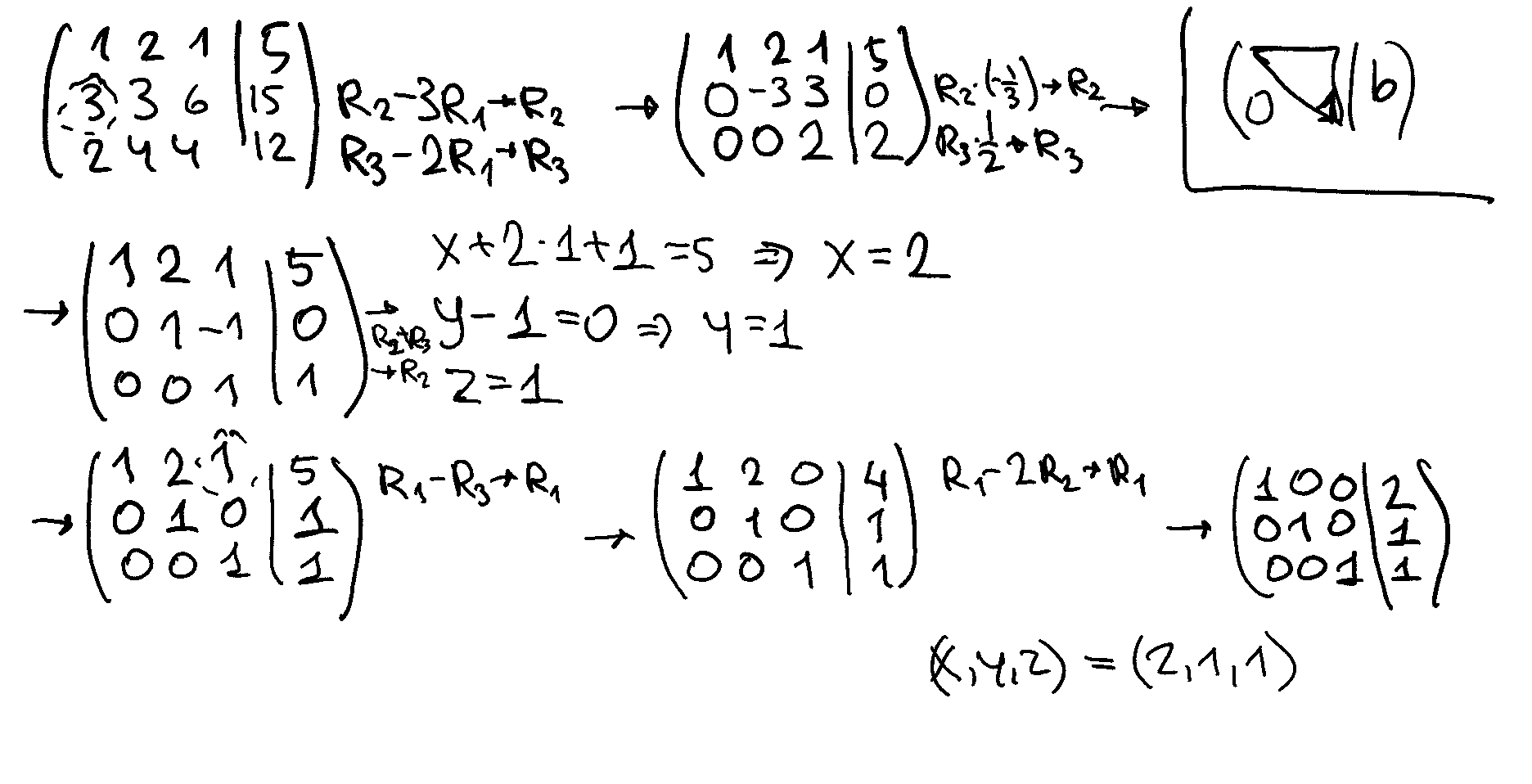
Hand written notes from the lecture

📖 Systems of linear equations

Contents

📖 Systems of linear equations#

What is a system of linear equations#

Gaussian elimination#

System with no solutions#

System with non-unique solutions#

Inverse by Gaussian row operations#

Solving a linear system using matrix inverse#

Determinants under Gaussian elimination#

Inverse by determinants#

Solving linear systems by determinants#

Notes from the lecture#