☕️ Numerical equation solving#
This chapter is for your information only, will not be part of the assessment
by Fedor Iskhakov
Description: Bisections and Newton-Raphson methods. Solving equations of one variable. Accuracy of solution. Rates of convergence.
YouTube recording of this lecture in the Foundational of Computational Economics course
Classic algorithm for equation solving#
Bisection method
Newton-Raphson method
Solve equations of the form \( f(x) = 0 \)
Focus on the scalar case today.
Bisection method for solving equations#
Solve equation \( f(x)=0 \), conditional on \( x \in [a,b] \subset \mathbb{R} \) such that \( f(a)f(b)<0 \)
Algorithm: similar to binary search, but in continuous space.
def bisection(f,a=0,b=1,tol=1e-6,maxiter=100,callback=None):
    '''Bisection method for solving equation f(x)=0
    on the interval [a,b], with given tolerance and number of iterations.
    Callback function is invoked at each iteration if given.
    '''
    if f(a)*f(b)>0:
        raise ValueError('Function has the same sign at the bounds')
    for i in range(maxiter):
        err = abs(b-a)
        if err<tol: break
        x = (a+b)/2
        a,b = (x,b) if f(a)*f(x)>0 else (a,x)
        if callback != None: callback(err=err,x=x,iter=i)
    else:
        raise RuntimeError('Failed to converge in %d iterations'%maxiter)
    return x
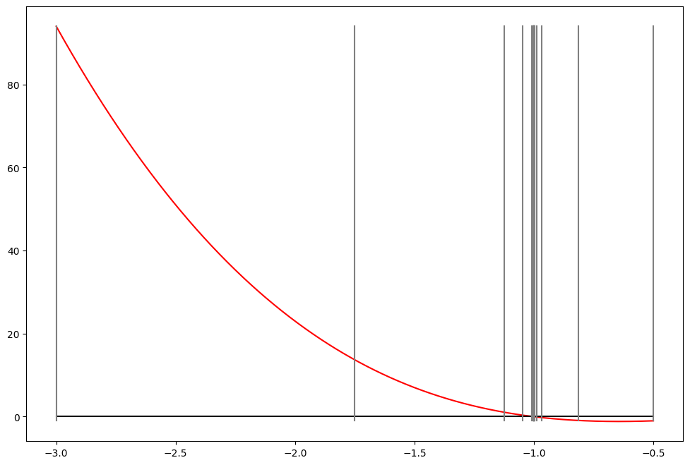
f = lambda x: -4*x**3+5*x+1
a,b = -3,-.5  # upper and lower limits
x = bisection(f,a,b)
print('Solution is x=%1.3f, f(x)=%1.12f' % (x,f(x)))
Solution is x=-1.000, f(x)=0.000000834465
# make nice plot
import numpy as np
import matplotlib.pyplot as plt
%matplotlib inline
plt.rcParams['figure.figsize'] = [12, 8]
xd = np.linspace(a,b,1000)  # x grid
plt.plot(xd,f(xd),c='red')  # plot the function
plt.plot([a,b],[0,0],c='black')  # plot zero line
ylim=[f(a),min(f(b),0)]
plt.plot([a,a],ylim,c='grey')  # plot lower bound
plt.plot([b,b],ylim,c='grey')  # plot upper bound
def plot_step(x,**kwargs):
    plot_step.counter += 1
    plt.plot([x,x],ylim,c='grey')
plot_step.counter = 0  # new public attribute
bisection(f,a,b,callback=plot_step)
print('Converged in %d steps'%plot_step.counter)
plt.show()
Converged in 22 steps
Newton-Raphson (Newton) method#
General form \( f(x)=0 \)
Equation solving
Finding maximum/minimum based on FOC, then \( f(x)=Q'(x) \)
Algorithm:
Start with some good guess \( x_0 \) not too far from the solution
Newton step: \( x_{i+1} = x_i - \frac{f(x_i)}{f'(x_i)} \)
Iterate until convergence in some metric
Derivation for Newton method using Taylor series expansion#
Take first two terms, assume \( f(x) \) is solution, and let \( x_0=x_i \) and \( x=x_{i+1} \)
def newton(fun,grad,x0,tol=1e-6,maxiter=100,callback=None):
    '''Newton method for solving equation f(x)=0
    with given tolerance and number of iterations.
    Callback function is invoked at each iteration if given.
    '''
    for i in range(maxiter):
        x1 = x0 - fun(x0)/grad(x0)
        err = abs(x1-x0)
        if callback != None: callback(err=err,x0=x0,x1=x1,iter=i)
        if err<tol: break
        x0 = x1
    else:
        raise RuntimeError('Failed to converge in %d iterations'%maxiter)
    return (x0+x1)/2
f = lambda x: -4*x**3+5*x+1
g = lambda x: -12*x**2+5
x = newton(f,g,x0=-2.5,maxiter=7)
print('Solution is x=%1.3f, f(x)=%1.12f' % (x,f(x)))
Solution is x=-1.000, f(x)=0.000000490965
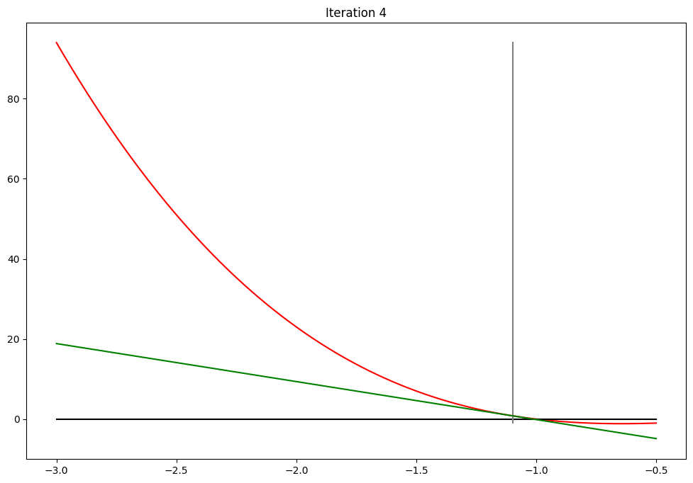
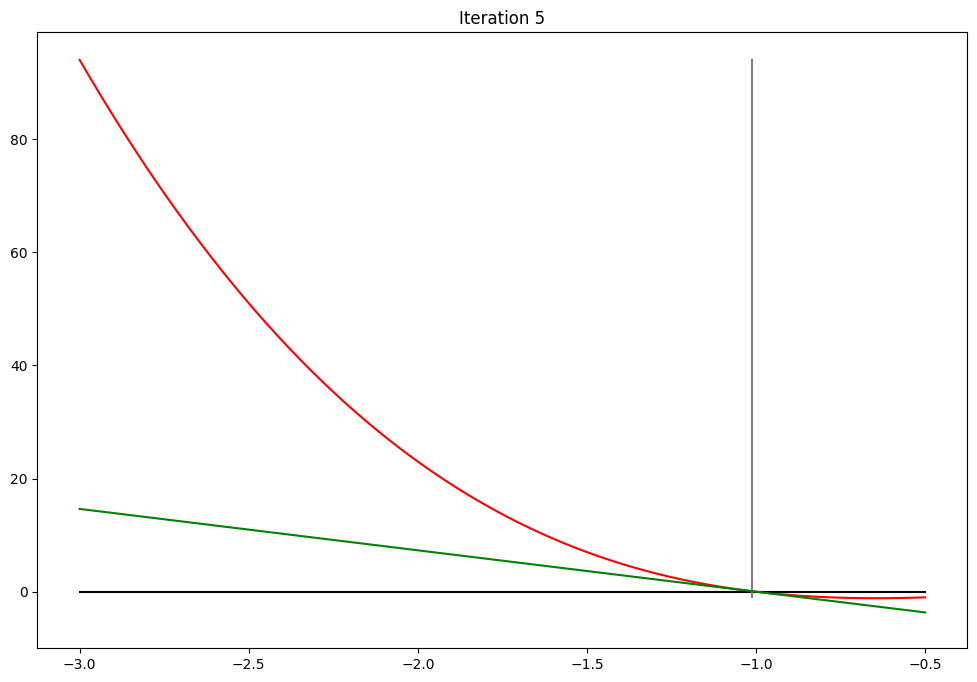
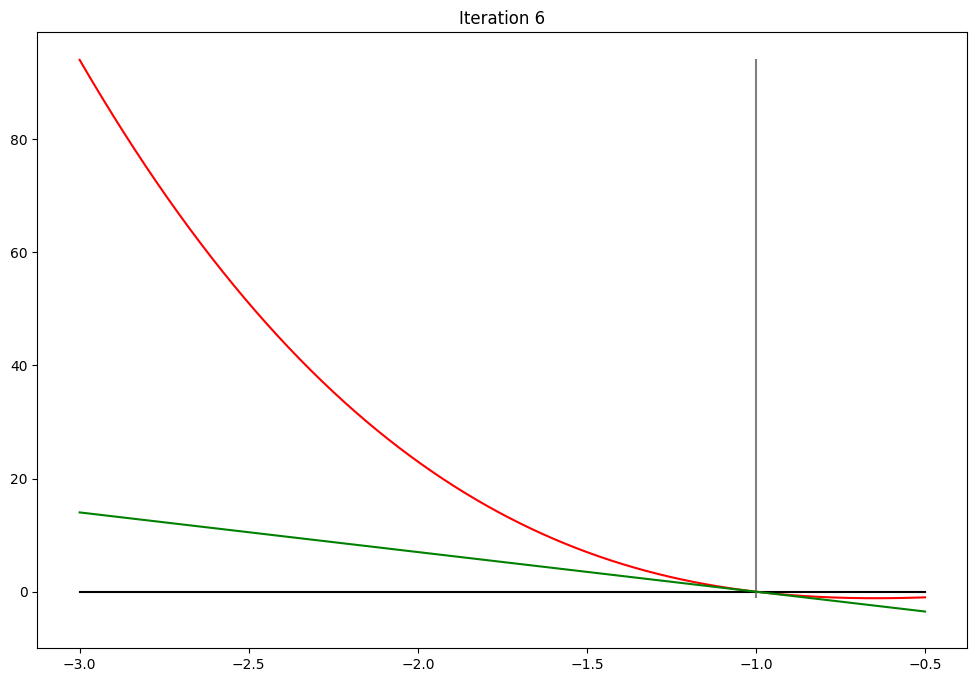
# make nice seriest of plots
a,b = -3,-.5  # upper and lower limits
xd = np.linspace(a,b,1000)  # x grid
def plot_step(x0,x1,iter,**kwargs):
    plot_step.counter += 1
    if iter<10:
        plt.plot(xd,f(xd),c='red')  # plot the function
        plt.plot([a,b],[0,0],c='black')  # plot zero line
        ylim = [min(f(b),0),f(a)]
        plt.plot([x0,x0],ylim,c='grey') # plot x0
        l = lambda z: g(x0)*(z - x1)
        plt.plot(xd,l(xd),c='green')  # plot the function
        plt.ylim(bottom=10*f(b))
        plt.title('Iteration %d'%(iter+1))
        plt.show()
plot_step.counter = 0  # new public attribute
newton(f,g,x0=-2.5,callback=plot_step)
print('Converged in %d steps'%plot_step.counter)
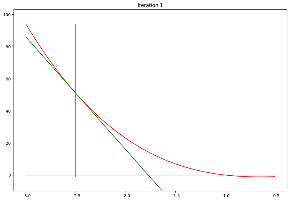

Converged in 7 steps
Rate of convergence of the two methods#
How fast does a solution method converge on the root of the equation?
Rate of convergence = the rate of decrease of the bias (difference between current guess and the solution)
Can be approximated by the rate of decrease of the error in the stopping criterion
Bisections: linear convergence
Newton: quadratic convergence
def print_err(iter,err,**kwargs):
    x = kwargs['x'] if 'x' in kwargs.keys() else kwargs['x0']
    print('{:4d}:  x = {:17.14f}  err = {:8.6e}'.format(iter,x,err))

print('Newton method')
newton(f,g,x0=-2.5,callback=print_err,tol=1e-10)

print('Bisection method')
bisection(f,a=-3,b=-0.5,callback=print_err,tol=1e-10)
Newton method
0: x = -2.50000000000000 err = 7.285714e-01
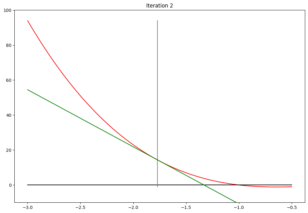
1: x = -1.77142857142857 err = 4.402791e-01
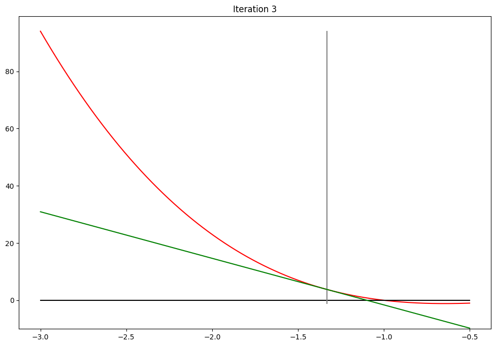
2: x = -1.33114944950557 err = 2.323743e-01
3: x = -1.09877514383983 err = 8.562251e-02
4: x = -1.01315263007170 err = 1.286646e-02
5: x = -1.00028616796687 err = 2.860277e-04
6: x = -1.00000014027560 err = 1.402756e-07
7: x = -1.00000000000003 err = 3.375078e-14
Bisection method
0: x = -1.75000000000000 err = 2.500000e+00
1: x = -1.12500000000000 err = 1.250000e+00
2: x = -0.81250000000000 err = 6.250000e-01
3: x = -0.96875000000000 err = 3.125000e-01
4: x = -1.04687500000000 err = 1.562500e-01
5: x = -1.00781250000000 err = 7.812500e-02
6: x = -0.98828125000000 err = 3.906250e-02
7: x = -0.99804687500000 err = 1.953125e-02
8: x = -1.00292968750000 err = 9.765625e-03
9: x = -1.00048828125000 err = 4.882812e-03
10: x = -0.99926757812500 err = 2.441406e-03
11: x = -0.99987792968750 err = 1.220703e-03
12: x = -1.00018310546875 err = 6.103516e-04
13: x = -1.00003051757812 err = 3.051758e-04
14: x = -0.99995422363281 err = 1.525879e-04
15: x = -0.99999237060547 err = 7.629395e-05
16: x = -1.00001144409180 err = 3.814697e-05
17: x = -1.00000190734863 err = 1.907349e-05
18: x = -0.99999713897705 err = 9.536743e-06
19: x = -0.99999952316284 err = 4.768372e-06
20: x = -1.00000071525574 err = 2.384186e-06
21: x = -1.00000011920929 err = 1.192093e-06
22: x = -0.99999982118607 err = 5.960464e-07
23: x = -0.99999997019768 err = 2.980232e-07
24: x = -1.00000004470348 err = 1.490116e-07
25: x = -1.00000000745058 err = 7.450581e-08
26: x = -0.99999998882413 err = 3.725290e-08
27: x = -0.99999999813735 err = 1.862645e-08
28: x = -1.00000000279397 err = 9.313226e-09
29: x = -1.00000000046566 err = 4.656613e-09
30: x = -0.99999999930151 err = 2.328306e-09
31: x = -0.99999999988358 err = 1.164153e-09
32: x = -1.00000000017462 err = 5.820766e-10
33: x = -1.00000000002910 err = 2.910383e-10
34: x = -0.99999999995634 err = 1.455192e-10
-0.9999999999563443
Measuring complexity of Newton and bisection methods#
What is the size of input \( n \)?
Desired precision of the solution!
Thus, attention to the errors in the solution as algorithm proceeds
Rate of convergence is part of the computational complexity of the algorithms
Computational complexity of Newton method#
Calculating a root of a function f(x) with n-digit precision
Provided that a good initial approximation is known
Is \( O((logn)F(n)) \), where \( F(n) \) is the cost of
calculating \( f(x)/f'(x) \) with \( n \)-digit precision
Further learning resources#
On computational complexity of Newton method https://m.tau.ac.il/~tsirel/dump/Static/knowino.org/wiki/Newton’s_method.html#Computational_complexity
“Improved convergence and complexity analysis of Newton’s method for solving equations” https://www.tandfonline.com/doi/abs/10.1080/00207160601173431?journalCode=gcom20