🔬 Tutorial problems zeta \(\zeta\)

Note

This problems are designed to help you practice the concepts covered in the lectures. Not all problems may be covered in the tutorial, those left out are for additional practice on your own.

\(\zeta\).1

Formulation

Using L’Hôpital’s rule compute the following limit

\[ \lim _{x \rightarrow \infty} \frac{x^{2}}{e^{x}} \]

Solution

Consider the function \(f(x)=\frac{g(x)}{h(x)}=\frac{x^{2}}{e^{x}}\). Note that

\[ \lim _{x \longrightarrow \infty} f(x)=\lim _{x \longrightarrow \infty} \frac{x^{2}}{e^{x}}=\frac{\lim _{x \longrightarrow \infty} x^{2}}{\lim _{x \longrightarrow \infty} e^{x}}=\frac{\infty}{\infty}, \]

which is of indeterminate form. We have \(g^{\prime}(x)=2 x\) and \(h^{\prime}(x)=e^{x}\). Note that

\[ \lim _{x \longrightarrow \infty} \frac{g^{\prime}(x)}{h^{\prime}(x)}=\lim _{x \longrightarrow \infty} \frac{2 x}{e^{x}}=\frac{\lim _{x \rightarrow \infty} 2 x}{\lim _{x \rightarrow \infty} e^{x}}=\frac{\infty}{\infty} \]

which is also of indeterminate form. We have \(g^{\prime \prime}(x)=2\) and \(h^{\prime \prime}(x)=e^{x}\). Note that

\[ \lim _{x \longrightarrow \infty} \frac{g^{\prime \prime}(x)}{h^{\prime \prime}(x)}=\lim _{x \longrightarrow \infty} \frac{2}{e^{x}}=\frac{\lim _{x \longrightarrow \infty} 2}{\lim _{x \longrightarrow \infty} e^{x}}=\frac{2}{\infty}=0 . \]

Thus we can conclude that

\[ \lim _{x \longrightarrow \infty} f(x)=\lim _{x \longrightarrow \infty} \frac{g(x)}{h(x)}=\lim _{x \longrightarrow \infty} \frac{x^{2}}{e^{x}}=\lim _{x \longrightarrow \infty} \frac{g^{\prime \prime}(x)}{h^{\prime \prime}(x)}=\lim _{x \longrightarrow \infty} \frac{2}{e^{x}}=0, \]

by L’Hopital’s rule.

\(\zeta\).2

Formulation

Consider function \(f \colon X \to \mathbb{R}\) defined by \(f(x) = \frac{1}{x} e^x\).

Find the minimizer(s) and the maximizer(s) of this function on \(X = (0, 2]\).

Follow all the required steps and explain your reasoning.

Hint

Review the algorithm for univariate optimization in the lecture notes

Solution

Following the algorithm for the univariate optimization from the lecture notes

1. Locate all stationary points

• according to the definition the stationary points are those interior points where \(f'(x) = 0\)

\[ f'(x) = \frac{d}{dx} \left( \frac{e^x}{x} \right) = \frac{e^x}{x} -\frac{1}{x^2} e^x = \frac{e^x}{x^2} \left( x - 1 \right) \]

\[ f'(x) =0 \iff x=1 \]

2. Evaluate the function at the stationary points and the boundaries, in our case only one boundary \(x=2\).

\[ f(1) = e \approx 2.718, \; f(2) = \frac{e^2}{2} \approx 3.694 \ \]

Evaluating the function at \(x=0\) is not possible because the function is not defined there! We have to be careful and investigate the behavior of the function as \(x\) approaches \(0\).

Because \(exp(x)\) is always positive, for small values of \(x\) the function takes on large numbers. The smaller \(x\) is, the larger the function becomes. This means that the function is unbounded as \(x\) approaches \(0\) (from the right). Therefore, we could move forward taking \(f(0) = \infty\).

3. Compare the values of the function at the stationary points and the boundaries to pick out the solution.

The minimizer of the function on \((0,2]\) is \(x=1\) because \(\min\{e,e^2/2,\infty\} = e\).

The maximizer of the function could be \(x=0\) because \(\max\{e,e^2/2,\infty\} = \infty\), but as the function is not defined at \(x=0\). We showed that the function grows without bound as \(x\) becomes closer and closer to 0, therefore it is impossible to find a precise \(x\) where it attains the maximum value (there is always possible to make a step towards zero to increase the function a little more). The conclusion is that there is no maximizer on \([0,2]\).

\(\zeta\).3

Formulation

Find an example of a nonlinear univariate function \(f \colon D \subset \mathbb{R} \to \mathbb{R}\) that:

(a) has exactly one maximizer and one minimizer (b) has has neither a maximizer nor a minimizer (c) has an infinite number of maximizers and minimizers (d) has exactly finite number \(n\) of maximizers and \(n\) minimizers

Remember to define both the function \(f(x)\) and its domain \(D\) for each case.

Hint

First, review the relevant definitions. Then, try to draft some ideas on a piece of paper. Think of how they can be expressed in mathematical terms.

Solution

This is a creative problem which has many possible correct answers.

As always, start with the definitions—in this case definitions of maximizer and minimizer.

Here is one possible solution:

(a) any linear (affine) function \(f(x)=ax+b\), \(a \ne 0\) on any close interval \([A,B]\) has no stationary points, and therefore exactly one maximizer and one minimizer at the edges of the interval.

(b) any linear (affine) function \(f(x)=ax+b\), \(a \ne 0\) on any open interval \((A,B)\) has no maximizer and no minimizer similarly to the no existence example in the lecture notes. A different idea would be to rely on positive and negative infinity in the domain \(D\), for example, let \(f(x) = \tan(\pi x)\) which takes values \(0\) on all integer points, and approaches a vertical line at every half-integer point.

(c) A constant function \(f(x) = C\) should immediately come to mind. Another possibility is the cyclic trigonometric functions like \(f(x) = \sin(x)\) or \(f(x) = \cos(x)\) on the entire real line. The latter only return values between -1 and 1, and attain these two values infinitely many times.

(d) This is the most tricky question, but one solution is to adjust the domain of the trig function such as \(f(x) = \cos(\pi x)\). This function attains 1 at \(x=\{...,-2,0,2,4,...\}\) and attains 0 at \(x=\{...,-3,-1,1,3,5,...\}\). Therefore, it has exactly \(n\) maximizers and \(n\) minimizers if we define \(D = [0,2n-1]\).

\(\zeta\).4

Formulation

A square tin plate whose edges are 18 cm long is to be made into an open square box of depth \(x\) cm by cutting out equally sized squares of width \(x\) in each corner and then folding over the edges. Draw a figure, and show that the volume of the box is, for \(x \in [0, 9]\):

\[ V(x) = x(18 - 2x)^2 = 4x^3 - 72x^2 + 324x \]

Also find maximum point of V in \([0, 9]\) and show it is indeed the maximum using second order conditions.

[Sydsæter, Hammond, Strøm, and Carvajal, 2016] Exercises for Section 8.3, Question 3

Hint

Solution

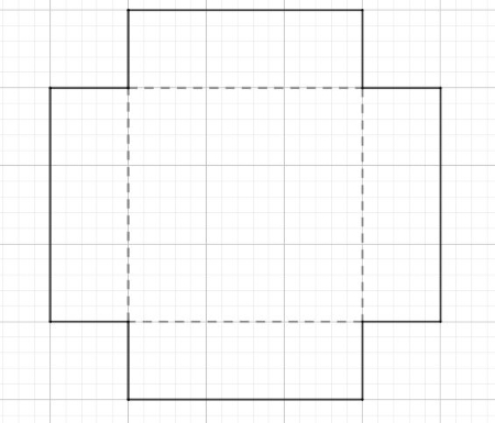
To avoid cutting out everything, we have to impose \(x<9\).

The volume is given by the product of width \(18-2x\) by length \(18-2x\) by height \(x\) of the box. This gives

\[ V(x) = x(18 - 2x)^2 = 4x^3 - 72x^2 + 324x \]

To find the maximum of \(V(x)\) differentiate and factorize:

\[ V'(x) = 12 x^2 - 144x + 324 = 12 (x^2 - 12x + 27) = 12 (x-3)(x-9) \]

The critical points are \(x=3\) and \(x=9\).

Applying the second order condition, compute \(V''(3)\), \(V''(9)\) and check their signs.

\[ V''(x) = 24 x - 144, \quad V''(3) = -72 >0 , \quad V''(3) = 72 > 0 \]

Therefore, at \(x=3\) there is a local maximum with \(V(3)=12 \cdot 12 \cdot 3 = 432\).

\(\zeta\).5

Formulation

The portion of families whose income is no more than \(x\), and who have a home computer, is given by

\[ p(x) = a + k (1-e^{-cx}), \]

where \(a\), \(k\), and \(c\) are positive constants. Determine \(p'(x)\) and \(p''(x)\). Does \(p(x)\) have a maximum? Sketch the graph of \(p(x)\) for \(x \geqslant 0\).

Solution

The first and second derivatives of \(p(x)\) are

\[ p'(x) = kc e^{-cx},\quad p''(x) = -kc^{2} e^{-cx} = -c p'(x) \]

Since \(kc > 0\), we have \(kce^{-cx} > 0\) for all \(x\). Thus, \(p'(x) > 0\) for all \(x\), which means that \(p(x)\) is increasing for all \(x\).

Similarly because \(c>0\) we have \(p''(x) < 0\) for all \(x\), which implies that \(p(x)\) is concave.

We can also note that \(p(x) < 1\) for all \(x \geqslant 0\) and therefore there it’s worth to compute the limit

\[ \lim_{x \to \infty} p(x) = \lim_{x \to \infty} \big(a + k(1 - e^{-cx})\big) = a + k(1 - 0) = a + k \]

With \(p(0) = a\) this is enough to sketch the graph of \(p(x)\) for \(x \geqslant 0\).

\(\zeta\).6

Formulation

Find the own price elasticity of demand for each of the following demand or inverse demand functions. If possible, find the price or prices for which the demand curves will: (i) be inelastic, (ii) have unitary elasticity and (iii) be elastic.

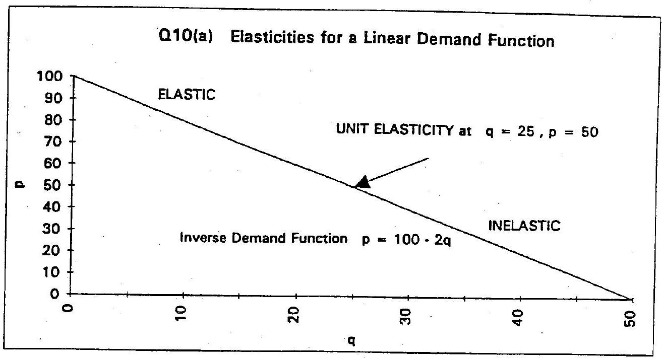
(a) \(P=100-2 Q\);

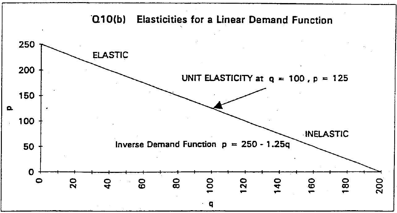
(b) \(Q=200-0.8 P\);

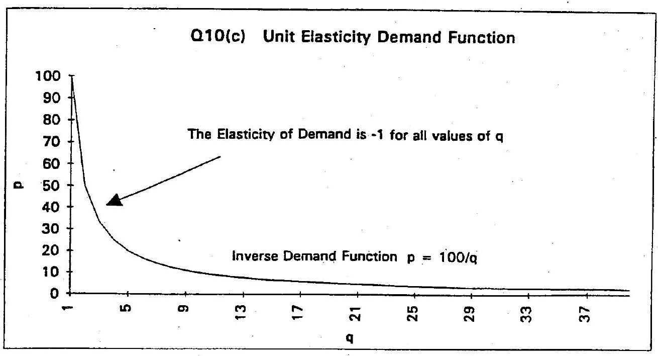
(c) \(P=100 Q^{-1}\);

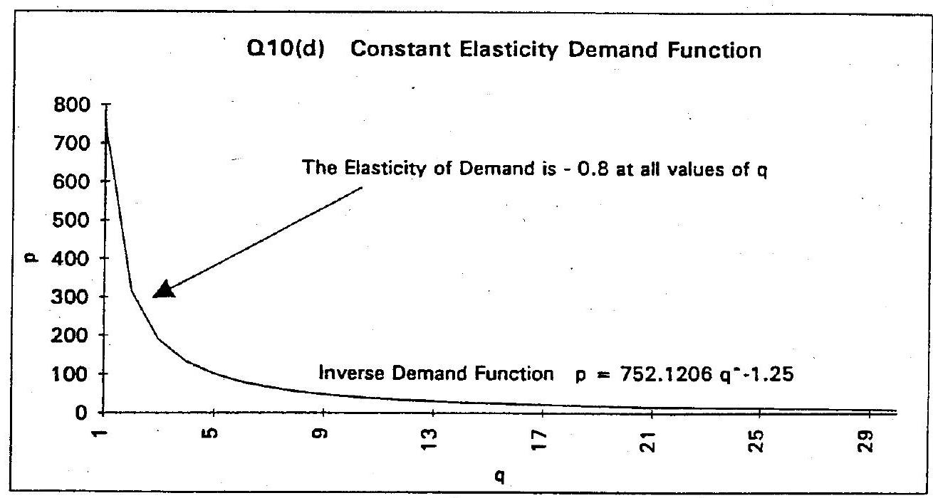
(d) \(Q=200 P^{-0.8}\);

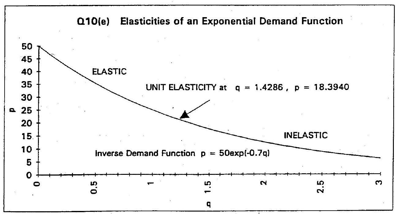
(e) \(P=50 e^{-0.7 Q}\); and

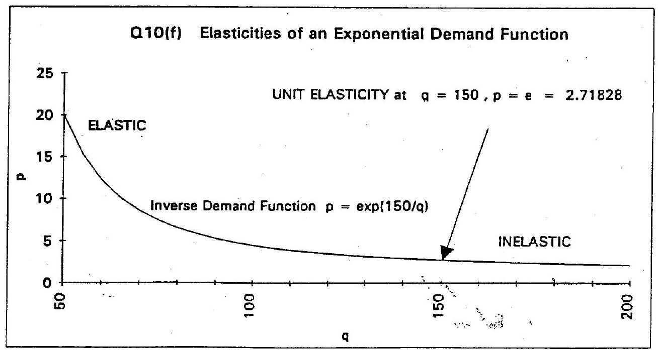
(f) \(Q=\frac{150}{\ln (P)}\).

[Shannon, 1995], p. 404

Solution

The answers to this question are directly drawn from the answer key to the exercises in Shannon (1995). This answer key was written by John Shannon and Ted McDonald. All figures presented here are also from that answer key.

The price elasticity of demand is defined in the following way

\[ \eta=\frac{d q}{d p} \cdot \frac{p}{q}=\frac{1}{\left(\frac{d p}{d q}\right)} \cdot \frac{p}{q} \]

For a linear demand function or a linear inverse demand function it is defined as

\[ \eta=b_{1} \cdot \frac{p}{q}=\frac{1}{\left(\frac{1}{b_{1}}\right)} \cdot \frac{p}{q} \]

(a)

For the inverse demand function \(p=100-2 q\) the derivative is

\[ \frac{\mathrm{dp}}{\mathrm{dq}}=-2 \]

and the price elasticity of demand is

\[ \eta=\frac{1}{-2} \frac{p}{q}=-\frac{p}{2 q} \]

To find where this demand curve has unit elasticity we let \(\eta=-1\) and find the values of \(p\) and \(q\) for which this is the case.

\[ -1=-\frac{p}{2 q} \]

Multiplying by \(-2 q\) gives the relationship which exists between \(p\) and \(q\) when there is unit elasticity.

\[ 2 q=p \]

We now substitute this expression for \(p\) into the inverse demand function

\[ 2 q=100-2 q \]

If we add \(2 q\) to both sides

\[ 4 q=100 \]

and then divide by 4 we obtain

\[ q=25 \]

To obtain \(p\) we use the relationship

\[\begin{split} \begin{array}{ll} p \quad & =2 q \\ & =50 \end{array} \end{split}\]

For this function we have \(\eta=-1\) when \(q=25\) and \(p=50\)

(b)

For the demand function

\[ q=200-0.8 p \]

we have

\[ \frac{\mathrm{dq}}{\mathrm{dp}}=-0.8 \]

and the price elasticity will be

\[ \eta=(-0.8) \frac{\mathrm{p}}{\mathrm{q}} \]

When \(\eta=-1\) then we will have

\[ -1=-0.8 \frac{p}{q} \]

and multiplying by \(-q\) gives

\[ q=0.8 p \]

Substituting this value of \(\mathrm{q}\) into the demand function gives

\[ 0.8 p=200-0.8 p \]

If we add .8 p we obtain

\[ 1.6 p=200 \]

and dividing by 1.6 gives

\[ \mathrm{p}=125 \]

Using the relationship between \(p\) and \(q\) we find

\[ \mathrm{q}=0.8 \mathrm{p}=100 \]

For this function we have \(\eta=-1\) when \(q=100\) and \(p=125\)

(c)

For the inverse demand function

\[ p=100 q^{-1} \]

we have

\[ \frac{d p}{d q}=-100 q^{-2} \]

and the price elasticity will be

\[\begin{split} \begin{array}{ll} \eta & =\frac{1}{-100 q^{-2}} \frac{p}{q}=\frac{q^{2}}{-100} \cdot \frac{p}{q} \\ & =-\frac{p q}{100} \end{array} \end{split}\]

Since \(p=100 q^{-1}\) we can write \(\eta\) as

\[ \eta=-\frac{100 q^{-1} q}{100}=-1 \]

For this type of function \(\eta=-1\) for any \(p\) and \(q\) values that lie on the inverse demand curve.

(d)

For the demand function

\[ q=200 p^{-0.8} \]

we have

\[ \frac{d q}{d p}=200\left(-0.8 p^{-1.8}\right)=-160 p^{-1.8} \]

and the price elasticity will be

\[ \eta=-160 p^{-1.8} \cdot \frac{p}{q}=-160 \frac{p^{-0.8}}{q} \]

Substituting \(q=200 p^{-0.8}\) into this expression gives

\[ \eta=\frac{-160 p^{-0.8}}{200 p^{-0.8}}=-0.8 \]

For this function \(\eta\) is always equal to -0.8 so no set of \(p\) and \(q\) values will make the value of \(\eta\) equal to -1 .

(e)

For the inverse demand function

\[ p=50 e^{-0.7 q} \]

we have

\[ \frac{d p}{d q}=50\left(-0.7 \cdot e^{-0.7 q}\right)=-35 e^{-0.7 q} \]

and the price elasticity will be

\[ \eta=\frac{1}{-35 e^{-0.7 q}} \cdot \frac{p}{q} \]

Substituting \(p=50 e^{-0.7 q}\) into this expression we obtain

\[ \eta=\frac{1}{-35 e^{-0.7 q}} \cdot \frac{50 e^{-0.7 q}}{q}=-\frac{10}{7 q} \]

When \(\eta=-1\) then

\[ -1=-\frac{10}{7 q} \]

and

\[ 7 q=10 \]

so

\[ q=\frac{10}{7} \]

Substituting this value of \(q\) into the inverse demand function gives

\[ \mathrm{p}=50 \cdot \mathrm{e}^{-0.7(10 / 7)}=50 \cdot \mathrm{e}^{-1}=18.3940 \]

For this function if \(\eta=-1\) when \(q=\frac{10}{7}\) and \(p=18.3940\).

(f)

For the demand function

we have

\[ q=150(\ln p)^{-1} \]

\[\begin{split} \begin{array}{ll} \frac{d q}{d p} & =150\left(-1(\ln p)^{-2}\left(\frac{1}{p}\right)\right) \\ & =\frac{-150}{(\ln p)^{2} \cdot p} \end{array} \end{split}\]

so

\[ \eta=\frac{-150}{(\ln p)^{2} \cdot p} \cdot \frac{p}{q} \]

Substituting \(q=150(\operatorname{ln} p)^{-1}\) into this expression gives

\[\begin{split} \begin{array}{ll} \eta & =\frac{-150}{(\ln p)^{2} 150(\ln p)^{-1}} \\ & =\frac{-1}{\ln p} \end{array} \end{split}\]

When \(\eta=-1\) then

\[ -1=-\frac{1}{\ln p} \]

and

\[ \ln p=1 \]

so that

\[ p=2.71828 \]

while

\[ \mathrm{q}=150(\ln \mathrm{p})^{-1}=150 \]

For this function we will have \(\eta=-1\) when \(q=150\) and \(p=2.71828\)