Announcements & Reminders

1. Next two weeks are teaching break 🎉

• March 31 to April 13

• No teaching

• No tutorials

• Good time to go over the material you struggle with, read the textbook and look through the extra material

2. Online test 2 next week on Thursday, April 3 😬

• covers material from the last three weeks

  • Sequences and convergence

  • Series

  • Limit of a function

  • Univariate differentiation

  • Applications of derivatives

• DO NOT FORGET

  • postponed tests only when validated by ANU’s procedure

• On short answer question write exactly what is asked

  • Single word is one and only on word!

  • Check your spelling

3. Two Fridays after the break are public holidays 🎊

• Lectures are recorded (see links in these notes)

• Tutorials proceed as usual, exercises for recorded lectures

• Next in-pension lecture is on May 2nd

2. Online test 3 after two weeks of recorded lectures on Thursday, May 1 😬

• covers material from the previous two weeks

  • Vector and matrix arithmetics

  • Linear systems of equations

• DO NOT FORGET

• On short answer question write exactly what is asked

Have a good break!

📖 Applications of derivatives

⏱ | words

References and additional materials

[Sydsæter, Hammond, Strøm, and Carvajal, 2016]

Chapters 7.12, 6.3, 8.7, 7.7, 7.10, 8 whole

L’Hôpital’s rule for indeterminate limits

Consider the function \(f(x)=\frac{g(x)}{h(x)}\).

Definition

If \(\lim _{x \rightarrow x_{0}} g(x)=\lim _{x \rightarrow x_{0}} h(x)=0\), we call this situation an “\(\frac{0}{0}\)” indeterminate form

If \(\lim _{x \rightarrow x_{0}} g(x)= \pm \infty\), \(\lim _{x \rightarrow x_{0}} h(x)= \pm \infty\), we call this situation an “\(\frac{ \pm \infty}{ \pm \infty}\)” indeterminate form

Fact: L’Hôpital’s rule for limits of indeterminate form

Suppose that \(g(x)\) and \(h(x)\) are both differentiable at all points on a non-empty interval \((a, b)\) that contains the point \(x=x_{0}\) (with the exception that they might not be differentiable at the point \(x_{0}\)).

Suppose also that \(h^{\prime}(x) \neq 0\) for all \(x \in(a, b)\).

Further, assume that for \(f(x)=\frac{g(x)}{h(x)}\) we have either “\(\frac{0}{0}\)” or “\(\frac{ \pm \infty}{ \pm \infty}\)” indeterminate form.

Then if \(\lim _{x \rightarrow x_{0}}\frac{g^{\prime}(x)}{h^{\prime}(x)}\) exists, then

\[ \lim _{x \rightarrow x_{0}} f(x) = \lim _{x \rightarrow x_{0}}\frac{g(x)}{h(x)} = \lim _{x \rightarrow x_{0}}\frac{g^{\prime}(x)}{h^{\prime}(x)} \]

• all four conditions have to hold for the L’Hôpital’s rule to hold!

Example

Note that in the examples below we have “\(\frac{0}{0}\)” indeterminacy, and both enumerator and denominator functions are differentiable around \(x=0\)

\[ \lim_{x \to 0} \frac{\ln(x+1)}{x} = \lim_{x \to 0} \frac{\frac{1}{x+1}}{1} = \lim_{x \to 0} \frac{1}{x+1} = 1 \]

\[ \lim_{x \to 0} \frac{e^x-1}{x} = \lim_{x \to 0} \frac{e^x}{1} = e^0 = 1 \]

Example

L’Hôpital’s rule is not applicable for \(\lim_{x \to 0} \frac{x}{\ln(x)}\) because neither “\(\frac{0}{0}\)” nor “\(\frac{ \pm \infty}{ \pm \infty}\)” indeterminacy form applies.

Example

For any \(p>0\) and \(a>1\) we have

\[ \lim_{x \to \infty} \frac{x^p}{a^x} = 0 \]

In other words any exponential function eventually grows faster than any power function!

Proof:

Consider logarithm of the ratio of the functions

\[ p \ln(x) - x \ln(a) = x\left(p\frac{\ln(x)}{x} - \ln(a)\right) \to \lim_{x \to \infty} x \left( \lim_{x \to \infty} \frac{\ln(x)}{x} - \ln(a) \right) \]

Clearly, \(\lim_{x \to \infty} x = \infty\).

With \(\lim_{x \to \infty} \frac{\ln(x)}{x}\) we have indeterminacy of the form \(\frac{\infty}{\infty}\), so by L’Hôpital’s rule

\[ \lim_{x \to \infty} \frac{\ln(x)}{x} = \lim_{x \to \infty} \frac{1/x}{1} = 0 \]

Coming back to the original limit, because \(\ln a>0\), we conclude that

\[ p \ln(x) - x \ln(a) = x\left(p\frac{\ln(x)}{x} - \ln(a)\right) \to -\infty \]

and therefore since \(\exp(y) \to 0\) as \(y \to -\infty\), \(\lim_{x \to \infty} \frac{x^p}{a^x} = 0\). \(\blacksquare\)

Investigating the shape of functions

First and second order derivatives are very useful for investigation the shape of functions.

Everywhere in this section we assume that \(A \subset \mathbb{R}\) is an open/semi-open/closed interval.

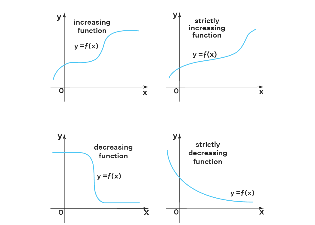
Increasing and decreasing functions

Definition

A function \(f : X \rightarrow \mathbb{R}\), where \(X \subseteq \mathbb{R}\), is said to be a non-decreasing (weakly increasing) function if

\[ x \leqslant y \iff f(x) \leqslant f(y) \]

Definition

A function \(f : X \rightarrow \mathbb{R}\), where \(X \subseteq \mathbb{R}\), is said to be a strictly increasing function if (a) \(x < y \iff f(x) < f(y)\).

Note the following:

• A strictly increasing function is also a one-to-one function.

• There are some one-to-one functions that are not strictly increasing.

• A strictly increasing function is also a non-decreasing function.

• There are some non-decreasing functions that are not strictly increasing.

Definition

Non-increasing and strictly decreasing functions are defined in a similar manner, with the inequality signs flipped.

Example

\[\begin{split} \begin{array}{ll} f(x) = x^3 & \text{is strictly increasing} \\ f(x) =\max\{x,5\} & \text{is increasing but not strictly} \\ f(x) = -\exp{x} & \text{is strictly decreasing} \\ f(x) = \sin{x} & \text{is neither increasing nor decreasing on } \mathbb{R} \\ f(x) = x+\sin{x} & \text{is strictly increasing (??)} \end{array} \end{split}\]

Desmos graph

Fact

For a differentiable function \(f: A\subset\mathbb{R} \to \mathbb{R}\), the following holds:

• \(f\) is non-decreasing \(\iff\) \(f'(x) \geqslant 0\) for all \(x \in A\)

• \(f\) is non-increasing \(\iff\) \(f'(x) \leqslant 0\) for all \(x \in A\)

• \(f\) is constant \(\iff\) \(f'(x) = 0\) for all \(x \in A\)

Example

\[ f(x) = x+\sin{x} \implies f'(x) = 1 + \cos{x} \geqslant 0 \; \text{for all}\; x \in \mathbb{R} \]

Therefore \(f\) is non-decreasing: adding \(g(x)=x\) to \(f(x)=\sin(x)\) is all it takes to stop the wiggling and make the function strictly increasing.

Fact

For a differentiable function \(f: A\subset\mathbb{R} \to \mathbb{R}\), the following holds:

• \(f\) is strictly increasing \(\impliedby\) \(f'(x) > 0\) for all \(x \in A\)

• \(f\) is strickly decreasing \(\impliedby\) \(f'(x) < 0\) for all \(x \in A\)

Note the equivalence (\(\iff\)) in the first fact and the implication (\(\impliedby\)) in the second fact

Unfortunately, there are examples when \(f'(x)=0\) and the function is still strictly decreasing or increasing

Example

\[ f(x) = x^3 \implies f'(x) = 3x^2 = 0 \; \text{when}\; x=0 \]

However, because the derivative comes on zero only ``momentarily’’, so even a smallest deviation from zero changes the function value in the right direction, \(f\) is strictly increasing around \(x=0\).

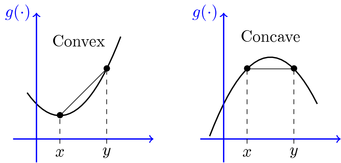
Concavity and convexity

Definition

Function \(f: A \subset \mathbb{R} \to \mathbb{R}\) is called convex if

\[ % f(\lambda x + (1 - \lambda) y) \leqslant \lambda f(x) + (1 - \lambda) f(y) % \]

for all \(x, y \in A\) and all \(\lambda \in [0, 1]\)

\(f\) is called strictly convex if

\[ % f(\lambda x + (1 - \lambda) y) < \lambda f(x) + (1 - \lambda) f(y) % \]

for all \(x, y \in A\) with \(x \ne y\) and all \(\lambda \in (0, 1)\)

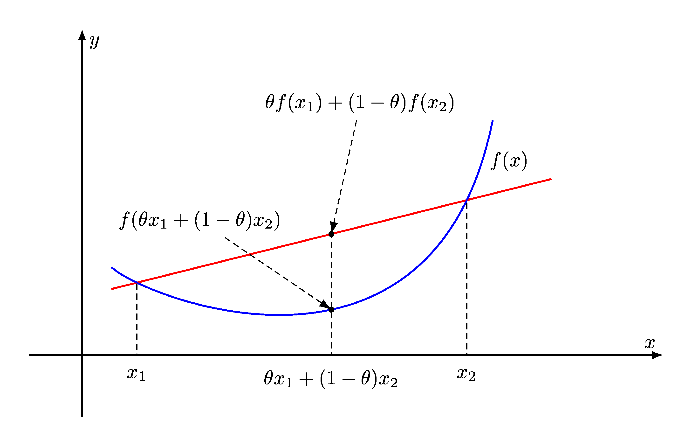
Definition

Function \(f: A \subset \mathbb{R} \to \mathbb{R}\) is called concave if

\[ f(\lambda x + (1 - \lambda) y) \geq \lambda f(x) + (1 - \lambda) f(y) \]

for all \(x, y \in A\) and all \(\lambda \in [0, 1]\)

\(f\) is called strictly concave if

\[ f(\lambda x + (1 - \lambda) y) > \lambda f(x) + (1 - \lambda) f(y) \]

for all \(x, y \in A\) with \(x \ne y\) and all \(\lambda \in (0, 1)\)

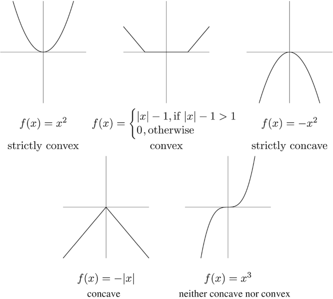
Example

Fact

\(f\) is concave if and only if \(-f\) is convex.

\(f\) is strictly concave if and only if \(-f\) is strictly convex

Proof

The inequality in the definitions flip with the sign change, so the result follows.

\(\blacksquare\)

Let \(f\) and \(g\) be functions from \(A \subset \mathbb{R}\) to \(\mathbb{R}\)

Fact

If \(f\) and \(g\) are convex (concave) and \(\alpha \geq 0\), then

• \(\alpha f\) is convex (concave)

• \(f + g\) is convex (concave)

If \(f\) and \(g\) are strictly convex (strictly concave) and \(\alpha > 0\), then

• \(\alpha f\) is strictly convex (strictly concave)

• \(f + g\) is strictly convex (strictly concave)

Proof

Let’s prove that \(f\) and \(g\) convex \(\implies h := f + g\) convex

Pick any \(x, y \in A\) and \(\lambda \in [0, 1]\)

We have

\[\begin{split} % & h(\lambda x + (1 - \lambda) y) = f(\lambda x + (1 - \lambda) y) + g(\lambda x + (1 - \lambda) y) \\ & \leqslant \lambda f(x) + (1 - \lambda) f(y) + \lambda g(x) + (1 - \lambda) g(y) \\ & = \lambda [f(x) + g(x)] + (1 - \lambda) [f(y) + g(y)] \\ & = \lambda h(x) + (1 - \lambda) h(y) % \end{split}\]

Hence \(h\) is convex \(\blacksquare\)

Derivatives (second derivative to be exact) help us to determine whether a function is convex or concave!

Fact

For a differentiable function \(f: A\subset\mathbb{R} \to \mathbb{R}\), the following holds:

• \(f\) is convex \(\iff\) \(f''(x) \geqslant 0\) for all \(x \in A\)

• \(f\) is concave \(\iff\) \(f''(x) \leqslant 0\) for all \(x \in A\)

Fact

For a differentiable function \(f: A\subset\mathbb{R} \to \mathbb{R}\), the following holds:

• \(f\) is strictly convex \(\impliedby\) \(f''(x) > 0\) for all \(x \in A\)

• \(f\) is strickly concave \(\impliedby\) \(f''(x) < 0\) for all \(x \in A\)

Again, note the equivalence (\(\iff\)) in the first fact and the implication (\(\impliedby\)) in the second fact

Unfortunately, there are examples when \(f''(x)=0\) and the function is still strictly concave or convex

Example

\[ f(x) = x^4 \implies f''(x) = 12x^2 = 0 \; \text{when}\; x=0 \]

However, because the second derivative comes on zero only ``momentarily’’, \(f\) is strictly convex around \(x=0\).

Example

• \(f(x) = a x + b\) is concave on \(\mathbb{R}\) but not strictly

• \(f(x) = \log(x)\) is strictly concave on \((0, \infty)\)

Example

• \(f(x) = a x + b\) is convex on \(\mathbb{R}\) but not strictly

• \(f(x) = x^2\) is strictly convex on \(\mathbb{R}\)

Show code cell content Hide code cell content

from myst_nb import glue
import matplotlib.pyplot as plt
import numpy as np

def subplots():
    "Custom subplots with axes through the origin"
    fig, ax = plt.subplots()
    # Set the axes through the origin
    for spine in ['left', 'bottom']:
        ax.spines[spine].set_position('zero')
    for spine in ['right', 'top']:
        ax.spines[spine].set_color('none')
    return fig, ax

xgrid = np.linspace(-2, 2, 200)
f = lambda x: (x**2-1)**2
fig, ax = subplots()
ax.set_ylim(-1, 2)
ax.set_yticks([-1, 1, 2])
ax.set_xticks([-1, 1])
ax.plot(xgrid, f(xgrid), 'k-', lw=2, alpha=0.8, label='$f=(x^2-1)^2$')
ax.plot([-1,-1], [-0.5,2], 'r:')
ax.plot([0,0], [-0.5,2], 'r:')
ax.plot([1,1], [-0.5,2], 'r:')
ax.plot([-1/np.sqrt(3),-1/np.sqrt(3)], [-0.5,2], 'b:')
ax.plot([1/np.sqrt(3),1/np.sqrt(3)], [-0.5,2], 'b:')
ax.legend(frameon=False, loc='lower right')
plt.show()
glue("square-square-example", fig, display=False)

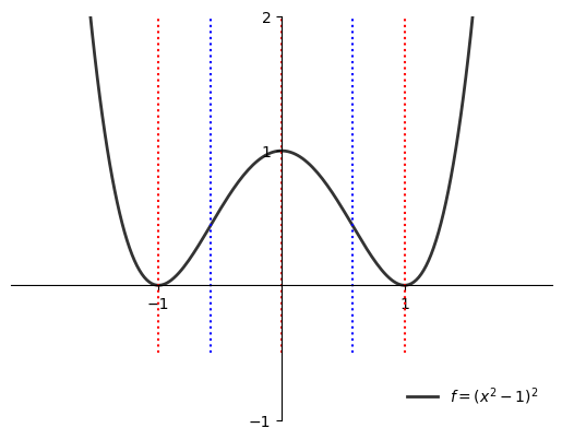
Example

Let’s investigate a shape of function \(f(x) = (x^2-1)^2\) on \(\mathbb{R}\).

The first and second derivatives are

\[ f'(x) = 4x(x^2-1)=4x(x-1)(x+1), \quad f''(x) = 4(3x^2-1) \]

Solving inequality \(f'(x) \geqslant 0\) gives

• when \(x \in (-\infty, -1] \cup [0, 1]\) \(f'(x) \leqslant 0\), thus the function is non-increasing on this set

• when \(x \in [-1,0] \cup [1,\infty)\) \(f'(x) \geqslant 0\), thus the function is non-decreasing on this set

Solving inequality \(f''(x) \geqslant 0\) gives

• when \(x \in (-\infty, -1/\sqrt{3}] \cup [1/\sqrt{3},\infty)\) \(f''(x) \geqslant 0\), thus the function is convex on this set

• when \(x \in [-1/\sqrt{3},1/\sqrt{3}]\) \(f''(x) \leqslant 0\), thus the function is concave on this set

Univariate optimization

Let \(f \colon [a, b] \to \mathbb{R}\) be a differentiable (smooth) function

• \([a, b]\) is all \(x\) with \(a \leqslant x \leqslant b\)

• \(\mathbb{R}\) is “all numbers”

• \(f\) takes \(x \in [a, b]\) and returns number \(f(x)\)

• derivative \(f'(x)\) exists for all \(x\) with \(a < x < b\)

Definition

A point \(x^* \in [a, b]\) is called a

• maximizer of \(f\) on \([a, b]\) if \(f(x^*) \geq f(x)\) for all \(x \in [a,b]\)

• minimizer of \(f\) on \([a, b]\) if \(f(x^*) \leqslant f(x)\) for all \(x \in [a,b]\)

Show code cell content Hide code cell content

from myst_nb import glue
import matplotlib.pyplot as plt
import numpy as np

def subplots():
    "Custom subplots with axes through the origin"
    fig, ax = plt.subplots()
    # Set the axes through the origin
    for spine in ['left', 'bottom']:
        ax.spines[spine].set_position('zero')
    for spine in ['right', 'top']:
        ax.spines[spine].set_color('none')
    return fig, ax

xmin, xmax = 2, 8
xgrid = np.linspace(xmin, xmax, 200)
f = lambda x: -(x - 4)**2 + 10

xstar = 4.0
fig, ax = subplots()
ax.plot([xstar], [0],  'ro', alpha=0.6)
ax.set_ylim(-12, 15)
ax.set_xlim(-1, 10)
ax.set_xticks([2, xstar, 6, 8, 10])
ax.set_xticklabels([2, r'$x^*=4$', 6, 8, 10], fontsize=14)
ax.plot(xgrid, f(xgrid), 'b-', lw=2, alpha=0.8, label=r'$f(x) = -(x-4)^2+10$')
ax.plot((xstar, xstar), (0, f(xstar)), 'k--', lw=1, alpha=0.8)
#ax.legend(frameon=False, loc='upper right', fontsize=16)
glue("fig_maximizer", fig, display=False)

xstar = xmax
fig, ax = subplots()
ax.plot([xstar], [0],  'ro', alpha=0.6)
ax.text(xstar, 1, r'$x^{**}=8$', fontsize=16)
ax.set_ylim(-12, 15)
ax.set_xlim(-1, 10)
ax.set_xticks([2, 4, 6, 10])
ax.set_xticklabels([2, 4, 6, 10], fontsize=14)
ax.plot(xgrid, f(xgrid), 'b-', lw=2, alpha=0.8, label=r'$f(x) = -(x-4)^2+10$')
ax.plot((xstar, xstar), (0, f(xstar)), 'k--', lw=1, alpha=0.8)
#ax.legend(frameon=False, loc='upper right', fontsize=16)
glue("fig_minimizer", fig, display=False)

xmin, xmax = 0, 1
xgrid1 = np.linspace(xmin, xmax, 100)
xgrid2 = np.linspace(xmax, 2, 10)

fig, ax = subplots()
ax.set_ylim(0, 1.1)
ax.set_xlim(-0.0, 2)
func_string = r'$f(x) = x^2$ if $x < 1$ else $f(x) = 0.5$'
ax.plot(xgrid1, xgrid1**2, 'b-', lw=3, alpha=0.6, label=func_string)
ax.plot(xgrid2, 0 * xgrid2 + 0.5, 'b-', lw=3, alpha=0.6)
ax.plot(xgrid1[-1], xgrid1[-1]**2, marker='o', markerfacecolor='white', markeredgewidth=2, markersize=6, color='b')
ax.plot(xgrid2[0], 0 * xgrid2[0] + 0.5, marker='.', markerfacecolor='b', markeredgewidth=2, markersize=10, color='b')
#ax.legend(frameon=False, loc='lower right', fontsize=16)
glue("fig_none", fig, display=False)

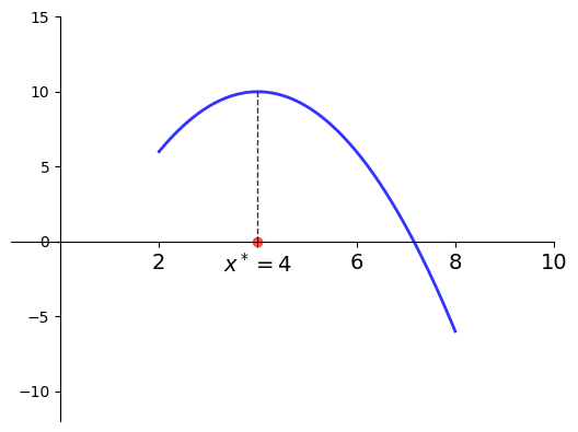
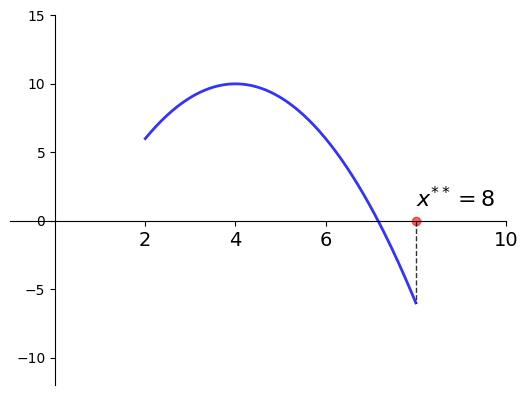
Example

Let

• \(f(x) = -(x-4)^2 + 10\)

• \(a = 2\) and \(b=8\)

Then

• \(x^* = 4\) is a maximizer of \(f\) on \([2, 8]\)

• \(x^{**} = 8\) is a minimizer of \(f\) on \([2, 8]\)

Fig. 31 Maximizer on \([a, b] = [2, 8]\) is \(x^* = 4\)

Fig. 32 Minimizer on \([a, b] = [2, 8]\) is \(x^{**} = 8\)

The set of maximizers/minimizers can be

• empty

• a singleton (contains one element)

• finite (contains a number of elements)

• infinite (contains infinitely many elements)

Example: infinite maximizers

\(f \colon [0, 1] \to \mathbb{R}\) defined by \(f(x) =1\)
has infinitely many maximizers and minimizers on \([0, 1]\)

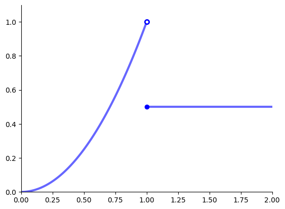
Example: no maximizers

The following function has no maximizers on \([0, 2]\)

\[\begin{split} f(x) = \begin{cases} x^2 & \text{ if } x < 1 \\ 1/2 & \text{ otherwise} \end{cases} \end{split}\]

Fig. 33 No maximizer on \([0, 2]\)

Definition

Point \(x\) is called interior to \([a, b]\) if \(a < x < b\)

The set of all interior points is written \((a, b)\)

We refer to \(x^* \in [a, b]\) as

• interior maximizer if both a maximizer and interior

• interior minimizer if both a minimizer and interior

Finding optima

Definition

A stationary point of \(f\) on \([a, b]\) is an interior point \(x\) with \(f'(x) = 0\)

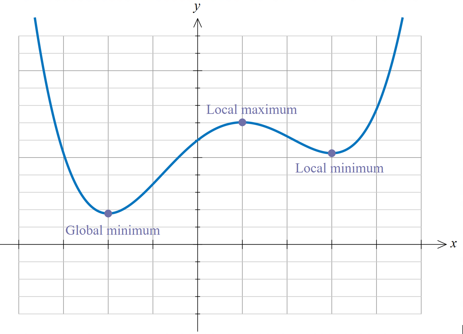
Fig. 34 Interior maximizers/minimizers are stationary points.

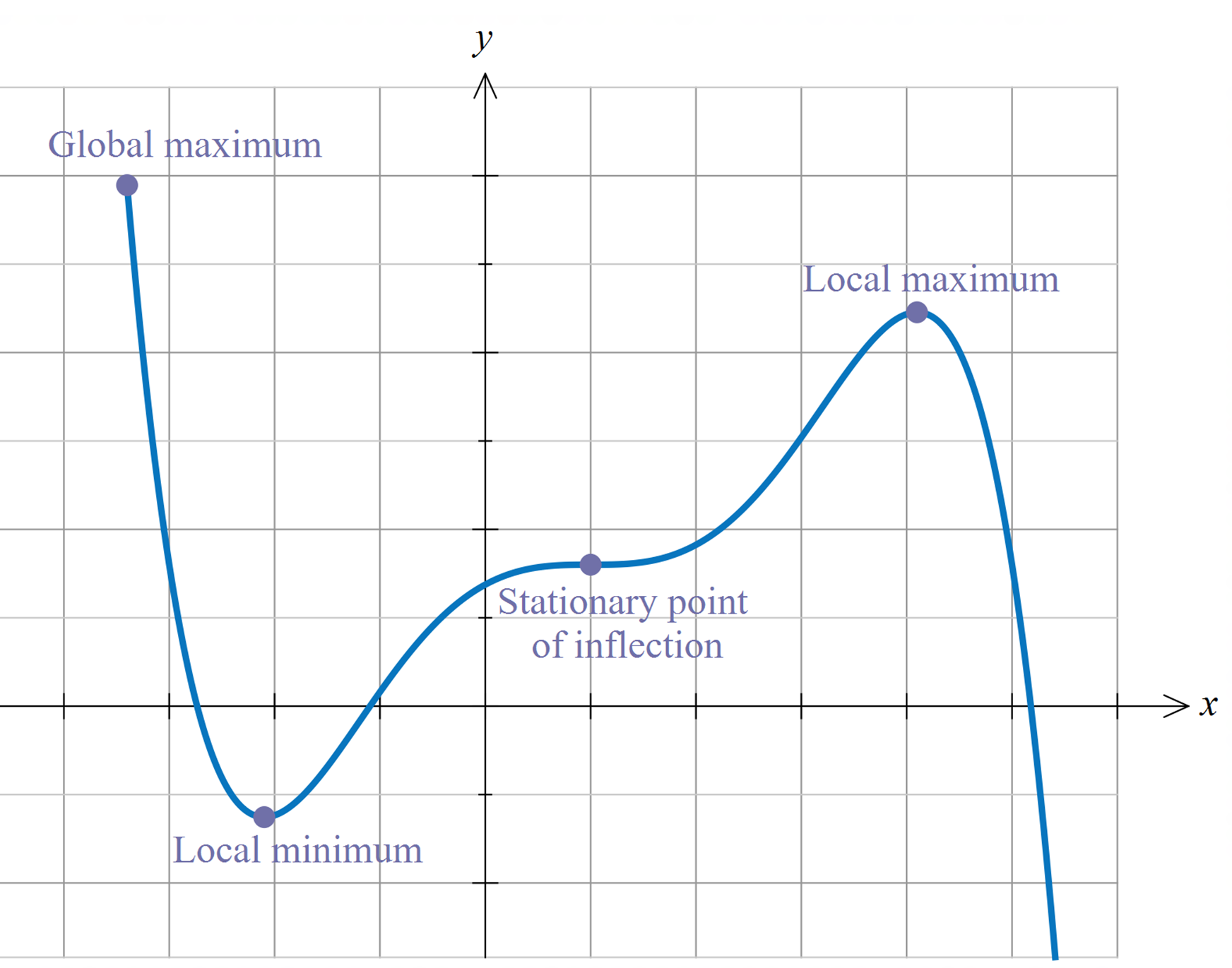
Fig. 35 Not all stationary points are maximizers!

Fact

If \(f\) is differentiable and \(x^*\) is either an interior minimizer or an interior maximizer of \(f\) on \([a, b]\), then \(x^*\) is stationary

Sketch of proof, for maximizers:

\[ f'(x^*) = \, \lim_{h \to 0} \, \frac{f(x^* + h) - f(x^*)}{h} \qquad \text{(by def.)} \]

\[ \Rightarrow f(x^* + h) \approx f(x^*) + f'(x^*) h \qquad \text{for small } h \]

If \(f'(x^*) \ne 0\) then exists small \(h\) such that \(f(x^* + h) > f(x^*)\)

Hence interior maximizers must be stationary — otherwise we can do better

Fact

Previous fact \(\implies\)

\(\implies\) any interior maximizer stationary
\(\implies\) set of interior maximizers \(\subset\) set of stationary points
\(\implies\) maximizers \(\subset\) stationary points \(\cup \{a\} \cup \{b\}\)

Algorithm for univariate problems

1. Locate stationary points

2. Evaluate \(y = f(x)\) for each stationary \(x\) and for \(a\), \(b\)

3. Pick point giving largest \(y\) value

Minimization: same idea

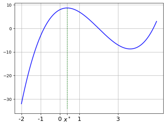
Example

Let’s solve

\[ \max_{-2 \leqslant x \leqslant 5} f(x) \quad \text{where} \quad f(x) = x^3 - 6x^2 + 4x + 8 \]

Steps

• Differentiate to get \(f'(x) = 3x^2 - 12x + 4\)

• Solve \(3x^2 - 12x + 4 = 0\) to get stationary \(x\)

• Discard any stationary points outside \([-2, 5]\)

• Eval \(f\) at remaining points plus end points \(-2\) and \(5\)

• Pick point giving largest value

from sympy import *
x = Symbol('x')
points = [-2, 5]
f = x**3 - 6*x**2 + 4*x + 8
fp = diff(f, x)
spoints = solve(fp, x)
points.extend(spoints)
v = [f.subs(x, c).evalf() for c in points]
maximizer = points[v.index(max(v))]
xstar = maximizer.evalf()
print("Maximizer =", str(maximizer),'=',xstar)

Maximizer = 2 - 2*sqrt(6)/3 = 0.367006838144548

Show code cell source Hide code cell source

import matplotlib.pyplot as plt
import numpy as np
xgrid = np.linspace(-2, 5, 200)
f = lambda x: x**3 - 6*x**2 + 4*x + 8
xstar=0.367006838144548
fig, ax = plt.subplots()
ax.plot(xgrid, f(xgrid), 'b-', lw=2, alpha=0.8)
ax.set_xticks([-2,-1,0,xstar,1,3])
yl=ax.get_ylim()
ax.set_xticklabels(['-2','-1','0',r'$x^*$','1','3'], fontsize=14)
ax.plot((xstar, xstar), (yl[0], f(xstar)), 'g--', lw=1, alpha=0.8)
ax.grid()

Second order conditions and local otpima

So far we have been talking about global maximizers and minimizers:

• definition in the very beginning

• algorithm above for univariate function on closed interval

It is important to keep in mind the desctinction between the global and local optima.

Definition

Consider a function \(f: A \to \mathbb{R}\) where \(A \subset \mathbb{R}^n\). A point \(x^* \in A\) is called a

• local maximizer of \(f\) if \(\exists \delta>0\) such that \(f(x^*) \geq f(x)\) for all \(x \in B_\delta(x^*) \cap A\)

• loca minimizer of \(f\) if \(\exists \delta>0\) such taht \(f(x^*) \leq f(x)\) for all \(x \in B_\delta(x^*) \cap A\)

In other words, a local optimizer is a point that is a maximizer/minimizer in some neighborhood of it and not necesserily in the whole function domain.

Fact (Second order conditions)

If \(f\) is twice differentiable and \(x^*\) is an interior point then

• if \(f'(x^*) = 0\) and \(f''(x^*) > 0\) then \(x^*\) is a local minimizer

• if \(f'(x^*) = 0\) and \(f''(x^*) < 0\) then \(x^*\) is a local maximizer

In univariate case the second order conditions amount to checking the sign of the second order derivative at the stationary point.

In higher dimensional cases the situation is much different. We will see how it works out in two dimensions in the end of the course.

Sufficiency and uniqueness with shape conditions

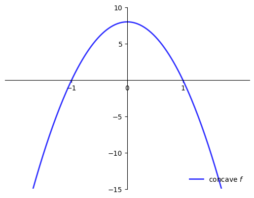
When is \(f'(x^*) = 0\) sufficient for \(x^*\) to be a maximizer?

One answer: When \(f\) is concave

Show code cell source Hide code cell source

xgrid = np.linspace(-2, 2, 200)
f = lambda x: - 8*x**2 + 8
fig, ax = subplots()
ax.set_ylim(-15, 10)
ax.set_yticks([-15, -10, -5, 5, 10])
ax.set_xticks([-1, 0, 1])
ax.plot(xgrid, f(xgrid), 'b-', lw=2, alpha=0.8, label='concave $f$')
ax.legend(frameon=False, loc='lower right')
plt.show()

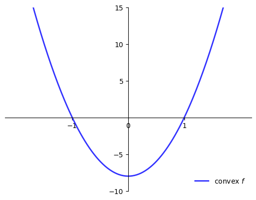
When is \(f'(x^*) = 0\) sufficient for \(x^*\) to be a minimizer?

One answer: When \(f\) is convex

Show code cell source Hide code cell source

xgrid = np.linspace(-2, 2, 200)
f = lambda x: - 8*x**2 + 8
fig, ax = subplots()
ax.set_ylim(-10, 15)
ax.set_yticks([-10, -5, 5, 10, 15])
ax.set_xticks([-1, 0, 1])
ax.plot(xgrid, -f(xgrid), 'b-', lw=2, alpha=0.8, label='convex $f$')
ax.legend(frameon=False, loc='lower right')
plt.show()

Fact

For maximizers:

• If \(f \colon [a,b] \to \mathbb{R}\) is concave and \(x^* \in (a, b)\) is stationary then \(x^*\) is a maximizer

• If, in addition, \(f\) is strictly concave, then \(x^*\) is the unique maximizer

Fact

For minimizers:

• If \(f \colon [a,b] \to \mathbb{R}\) is convex and \(x^* \in (a, b)\) is stationary then \(x^*\) is a minimizer

• If, in addition, \(f\) is strictly convex, then \(x^*\) is the unique minimizer

Show code cell content Hide code cell content

p = 2.0
w = 1.0
alpha = 0.6
xstar = (alpha * p / w)**(1/(1 - alpha))
xgrid = np.linspace(0, 4, 200)
f = lambda x: x**alpha
pi = lambda x: p * f(x) - w * x
fig, ax = subplots()
ax.set_xticks([1,xstar,2,3])
ax.set_xticklabels(['1',r'$\ell^*$','2','3'], fontsize=14)
ax.plot(xgrid, pi(xgrid), 'b-', lw=2, alpha=0.8, label=r'$\pi(\ell) = p\ell^{\alpha} - w\ell$')
ax.plot((xstar, xstar), (0, pi(xstar)), 'g--', lw=1, alpha=0.8)
#ax.legend(frameon=False, loc='upper right', fontsize=16)
glue("fig_price_taker", fig, display=False)
glue("ellstar", round(xstar,4))

Example

A price taking firm faces output price \(p > 0\), input price \(w >0\)

Maximize profits with respect to input \(\ell\)

\[ \max_{\ell \ge 0} \pi(\ell) = p f(\ell) - w \ell, \]

where the production technology is given by

\[ f(\ell) = \ell^{\alpha}, 0 < \alpha < 1. \]

Evidently

\[ \pi'(\ell) = \alpha p \ell^{\alpha - 1} - w, \]

so unique stationary point is

\[ \ell^* = (\alpha p/w)^{1/(1 - \alpha)} \]

Moreover,

\[ \pi''(\ell) = \alpha (\alpha - 1) p \ell^{\alpha - 2} < 0 \]

for all \(\ell \ge 0\) so \(\ell^*\) is unique maximizer.

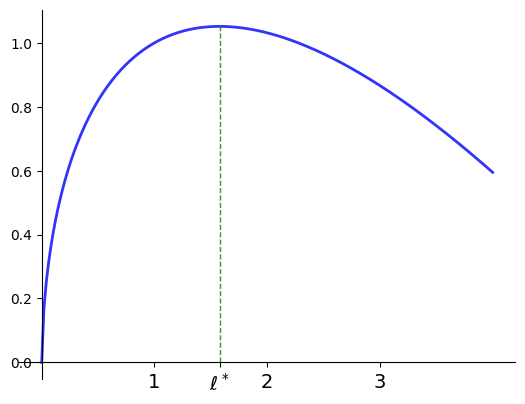
Fig. 36 Profit maximization with \(p=2\), \(w=1\), \(\alpha=0.6\), \(\ell^*=\)1.5774

Elasticity

Elasticity and in particular point elasticity is a concept that is widely used in economics for measuring responsiveness of economic quantities (demand, labor supply, etc.) to changes in other economic quantities (prices, wages, etc.)

Definition (in words)

Suppose that \(y=f(x)\). The elasticity of \(y\) with respect to \(x\) is defined to be the percentage change in \(y\) that is induced by a small (infinitesimal) percentage change in \(x\).

So, what is a percentage change in \(x\)?

• \(x\) to \(x+h\), making \(h\) the absolute change in \(x\)

• \(x\) to \(x + rx\), making \((x+rx)/x = 1+r\) the relative change in \(x\), and \(r\) is the relative change rate

• percentage change in \(x\) is the relative change rate expressed in percentage points

We are interested in infinitesimal percentage change, therefore in the limit as \(r \to 0\) (irrespective of the units of \(r\))

What is the percentage change in \(y\)?

Answer: rate of change of \(f(x)\) that can be expressed as

\[ \frac{f(x+rx)}{f(x)} -1 = \frac{f\big(x(1+r)\big)-f(x)}{f(x)} \]

Let’s consider the limit

\[ \lim_{r \to 0} \frac{\frac{f\big(x(1+r)\big)-f(x)}{f(x)}}{r} = \frac{1}{f(x)} \lim_{r \to 0} \frac{f\big(x(1+r)\big)-f(x)}{r} = \]

Define a new function \(g\) such that \(f(x) = g\big(\ln(x)\big)\) and \(f\big(x(1+r)\big) = g\big(\ln(x) + \ln(1+r)\big)\)

Continuing the above, and noting that \(\ln(1+r) \to 0\) as \(r \to 0\) we have

\[\begin{split} \begin{array}{l} = \frac{1}{f(x)} \lim_{r \to 0} \frac{g\big(\ln(x) + \ln(1+r)\big)-g\big(\ln(x)\big)}{r} = \\ = \frac{1}{f(x)} \lim_{r \to 0} \frac{g\big(\ln(x) + \ln(1+r)\big)-g\big(\ln(x)\big)}{\ln(1+r)} \frac{\ln(1+r)}{r} = \\ = \frac{1}{f(x)} \left[ \lim_{r \to 0} \frac{g\big(\ln(x) + \ln(1+r)\big)-g\big(\ln(x)\big)}{\ln(1+r)} \lim_{r \to 0} \frac{\ln(1+r)}{r} \right] =\\= \frac{1}{f(x)} \frac{d g(\ln(x))}{d \ln(x)} = \frac{1}{f(x)} \frac{d f(x)}{d \ln(x)} = \frac{x}{f(x)} \frac{d f(x)}{d x} \end{array} \end{split}\]

See the example above showing that \(\lim_{r \to 0} \frac{\ln(1+r)}{r} = 1\).

In the last step, to make sense of the expression \(\frac{d f(x)}{d \ln(x)}\), imagine that \(x\) is a function of some other variable we call \(\ln(x)\). Then we can use the chain rule and the inverse function rule to show that

\[ \frac{d f(x)}{d \ln(x)} = \frac{d f(x)}{d x} \frac{dx}{d \ln(x)} = \frac{d f(x)}{d x} \frac{1}{\frac{1}{x}} = x \frac{d f(x)}{d x} \]

Note, in addition, that by the chain rule the following also holds

\[ \frac{d \ln f(x)}{d \ln(x)} = \frac{1}{f(x)} \frac{d f(x)}{d \ln(x)} \]

Putting everything together, we arrive at the following equivalent expressions for elasticity.

Definition (exact)

The (point) elasticity of \(f(x)\) with respect to \(x\) is defined to be the percentage change in \(y\) that is induced by a small (infinitesimal) percentage change in \(x\), and is given by

\[ \epsilon^{f}_{x}(x)= \lim_{r \to 0} \frac{\frac{f\big(x(1+r)\big)}{f(x)}-1}{r} = \frac{\frac{d f(x)}{d x}}{\frac{f(x)}{x}} = \frac{x}{f(x)} \frac{d f(x)}{d x} = \frac{d \ln f(x)}{d \ln x} \]

Example

Suppose that we have a linear demand curve of the form

\[ Q = a − bP \]

where \(a > 0\) and \(b > 0\) The slope of this demand curve is equal to \((−b)\) As such, the point own-price elasticity of demand in this case is given by

\[\begin{split} \begin{align*} \epsilon^D_P (P) &= \left( \frac{P}{a - bP} \right) (-b) \\ &= \left( \frac{-bP}{a - bP} \right) \end{align*} \end{split}\]

Note that

\[\begin{split} \begin{align*} | \epsilon^D_P (P) | &= 1 \\ \iff | \frac{-bP}{a - bP} | &= 1 \\ \iff \frac{bP}{a - bP} &= 1 \\ \iff bP &= a - bP \\ \iff 2bP &= a \\ \iff P &= \frac{a}{2b} \\ \end{align*} \end{split}\]

More generally, we can show that, for the linear demand curve above, we have

\[\begin{split} | \epsilon^D_P (P) | = \begin{cases} \in (0, 1) \;\; \text{ if } P < \frac{a}{2b} \\ = 1 \;\; \text{ if } P = \frac{a}{2b} \\ \in (1, \infty) \;\; \text{ if } P > \frac{a}{2b} \\ \end{cases} \end{split}\]

Since the demand curve above is downward sloping, this means that

\[\begin{split} \epsilon^D_P (P) = \begin{cases} \in (-1, 0) \;\; \text{ if } P < \frac{a}{2b} \\ = -1 \;\; \text{ if } P = \frac{a}{2b} \\ \in (-\infty, -1) \;\; \text{ if } P > \frac{a}{2b} \\ \end{cases} \end{split}\]

Example

Suppose that we have a demand curve of the form

\[ Q = a/P \]

where \(a > 0\). Computing the point elasticity of demand at price \(P\) we have

\[\begin{split} \begin{align*} \epsilon^D_P (P) &= \left( \frac{P}{a/P} \right) \left( \frac{-a}{P^2} \right) \\ &= \frac{P^2}{a}\frac{-a}{P^2} = -1 \end{align*} \end{split}\]

Constant own-price elasticity!

Alternatively we could compute this elasticity as

\[\begin{split} Q &= a/P = a P^{-1} \quad \Leftrightarrow \quad \ln Q = \ln a - \ln P \\ \epsilon^D_P (P) &= \frac{d \ln Q}{d \ln P} = -1 \end{split}\]

Newton-Raphson method

Classic method for fast numerical solving the equation of the form \(f(x)=0\)

• Equation solving

• Finding maximum/minimum based on FOC, then \( f(x)=Q'(x)\)

• Quadratic convergence rate when initialized in the domain of attraction of the solution

Algorithm:

1. Start with some good guess \( x_0 \) not too far from the solution

2. Newton step: \( x_{i+1} = x_i - \frac{f(x_i)}{f'(x_i)} \)

3. Iterate until convergence in some metric

Derivation based on the Taylor series

\[ f(x) = \sum_{k=0}^{\infty} \frac{f^{(k)}(x_0)}{k!} (x-x_0)^k \]

Take first two terms, assume \( f(x) \) is solution, and let \( x_0=x_i \) and \( x=x_{i+1} \)

\[ 0 = f(x) = f(x_i) + f'(x_i) (x_{i+1}-x_i) \quad \Rightarrow \quad x_{i+1} = x_i - \frac{f(x_i)}{f'(x_i)} \]

Example

See the working example in Jupyter Notebook