Announcements & Reminders
Tutorials start(ed) this week
Make sure you register for tutorials on course pages
Reminder on how to ask questions:
Administrative: RSE admin
Content/understanding: tutors
Other: to Fedor
You may be interested in this event on March 6

📖 Sets and numbers#
⏱ | words
References and additional materials
[Sydsæter, Hammond, Strøm, and Carvajal, 2016]
Chapters 1.1, 2.1-2.5
Veritasium video on paradoxes of set theory and mathematical incompleteness YouTube
Notation cheat sheet
Notation |
Meaning |
|---|---|
\(P \implies Q\) |
\(P\) implies \(Q\) |
\(P \iff Q\) |
\(P \implies Q\) and \(Q \implies P\) |
\(\exists\) |
there exists |
\(\forall\) |
for all [elements in a set] |
\(a := \text{[expression]}\) |
\(a\) is defined to be equal to \(\text{[expression]}\) |
\(a \equiv \text{[expression]}\) |
\(a\) is defined to be equal to \(\text{[expression]}\) |
\(a \stackrel{def.}{=} \text{[expression]}\) |
\(a\) is defined to be equal to \(\text{[expression]}\) |
\(\in\) |
is element of |
\(\subset\) |
is subset of |
\(\cup\) |
union |
\(\cap\) |
intersection |
Naive set theory#
Definition
A set (\(X\)) is a collection of objects.
A particular object within a set (\(x\)) is known as an element of that set.
Sets: \(A, B, X\)
Elements: \(x,y,z\)
\(x \in X\) denotes the idea that x is an element of X
\(y \notin X\) denotes the idea that y is not an element of X
empty set is denoted by \(\varnothing\)
Definition of a set
A set \(A\) can be defined by either
direct enumeration of its elements
defining a formula for infinite number of elements
as a subset of already defined set \(B\), formula \(\psi(x)\) to form elements of \(A\), and a condition/property on \(x\)
The idea that x is an element of X is written in mathematical notation as \(x \in X\).
Suppose that there are elements that do not belong to \(X\). Let \(y\) be one such element. The idea that \(y\) is not an element of \(X\) is written in mathematical notation as \(y \notin X\) .
A set that does not contain any elements is said to be empty. An empty set is denoted by either \(\varnothing\) or \(\{\}\).
There are two fundamental ways of defining a particular set:
The first of these is to exhaustively list all of the elements of the set.
Example 1: \(X = \{1, 2, 3\}\)
Example 2: \(Y = \{1, 2, 3, · · · , 100\}\)
Example 3: \(\mathbb{N} = \{1, 2, 3, · · · \}\)
The second of these is to specify one or more properties that characterise all of the elements in the set.
Example 4: \(X = \{n \in \mathbb{N} : n < 4\}\)
Example 5: \(Y = \{n \in \mathbb{N} : n \leqslant 100\}\)
Some common number sets#
The set of natural numbers:
The set of non-negative intergers:
The set of integers:
The set of rational numbers:
The set of non-negative rational numbers:
The set of positive rational numbers:
The set of real numbers:
The set of non-negative real numbers:
The set of positive real numbers:
The set of complex numbers:
Example
Non-negative and positive real orthants#
The set of non-negative real numbers is given by
The Euclidean \(L\)-dimensional non-negative orthant is
The set of positive real numbers is given by
The Euclidean \(L\)-dimensional positive orthant is
Non-positive and negative real orthants#
The set of non-positive real numbers is given by
The Euclidean \(L\)-dimensional non-positive orthant is
The set of negative real numbers is given by
The Euclidean \(L\)-dimensional negative orthant is
Subsets#
Definition
Consider two sets, \(X\) and \(Y\). Suppose that every element of \(X\) also belongs to \(Y\). If this is the case, then we say that \(X\) is a subset of \(Y\).
This is written in mathematical notation as \(X \subseteq Y\).
Definition
Suppose that in addition to every element of \(X\) also belonging to \(Y\), there is at least one element of Y that does not belong to \(X\). If this is the case, then we say that \(X\) is a proper subset of \(Y\).
This is written is mathematical notation as \(X \subset Y\).
Sometimes \(X \subset Y\) is used (rather loosely) to mean \(X \subseteq Y\). If this meaning of the notation is employed, then \(X \subsetneq Y\) would need to be used to indicate that \(X\) is a proper subset of \(Y\).
Suppose that both every element of \(X\) also belongs to \(Y\), and every element of \(Y\) also belongs to \(X\). If this is the case, then we say that \(X\) is equal to \(Y\). This is written in mathematical notation as \(X = Y\).
The nesting of number sets#
Example
Recall the common number sets from above. The following “nesting” relationship exists between these common sets of numbers:
Note that \(\mathbb{N} \subset \mathbb{Z}_+\) because \(\mathbb{Z}_+ = \mathbb{N} \cup \{0\}\).
Note that \(\mathbb{Z}_+ \subset \mathbb{Z}\) because \(\mathbb{Z} = \mathbb{Z}_+ \cup \{ · · · , −3, −2, −1 \}\).
Note that \(\mathbb{Z} \subset \mathbb{Q}\) because any \(m \in \mathbb{Z}\) can be written as \(\frac{m}{1}\) and \(1 \in \mathbb{N}\), but there are fractions that do not belong to Z (for example \(\frac{1}{2} \notin \mathbb{Z}\)).
Note that \(\mathbb{Q} \subset \mathbb{R}\) because \(\frac{m}{n} \in (−\infty, \infty)\) for all \(m \in \mathbb{Z}\) and \(n \in \mathbb{N}\), but there are numbers on the real line that cannot be expressed as fractions (for example \(\sqrt{2}\), \(\pi\) and \(e\)). Real numbers that cannot be expressed as fractions are known as “irrational numbers”.
Note that \(\mathbb{R} \subset \mathbb{C}\) because
and \(0 \in \mathbb{R}\), but \((a + bi) \notin \mathbb{R}\) if \(b \neq 0\).
Complex numbers in which a = 0 are known as (purely) “imaginary numbers”.
Intervals as subsets of the real line#
Some (but not all) of the subsets of the real line take the form of an interval.
Let \(a \in \mathbb{R}, b \in \mathbb{R} \text{ and } a \le b\). There are four types of intervals:
\([a, b] = \{x \in \mathbb{R} : a \leqslant x \leqslant b\}\)
If \(a > b\), then \([a, b] = \varnothing\)
If \(a = b\), then \([a, b] = \{a\} = \{b\}\)
\((a, b) = \{x \in \mathbb{R} : a < x < b\}\)
If \(a > b\), then \((a, b) = \varnothing\)
If \(a = b\), then \((a, b) = \varnothing\)
\([a, b) = \{x \in \mathbb{R} : a \leqslant x < b\}\)
If \(a > b\), then \([a, b) = \varnothing\)
\((a, b] = \{x \in \mathbb{R} : a < x \leqslant b\}\)
If \(a > b\), then \((a, b] = \varnothing\)
Power sets#
Definition
The power set \(2^X\) of a set \(X\) is the set of all subsets of \(X\).
Note that the elements of a power set are sets themselves.
If there are \(n < \infty\) elements (that is, a finite number of elements) in the set \(X\), then the number of subsets of \(X\) will be equal to \(2^n\). As such, there will be \(2^n\) elements in the set \(2^X\). This might be the reason that the power set for some set \(X\) is often denoted by \(2^X\).
Example
Suppose that \(X = \{1, 2, 3\}\). The power set for the set \(X\) in this example is
Note that there are three elements in the set \(X\) and eight elements in the power set for \(X\), \(2^3 = 8\).
Cartesian product#
Definition
The Cartesian product of two sets is defined to be the set of all ordered pairs (or doublets) that contain one component from each of the two sets in the order that the sets were specified. This can be formally expressed as
Definition
The Cartesian product of \(n\) sets is defined to be the set of all ordered \(n\)-tuples that contain one component from each of the \(n\) sets in the order that the sets were specified. This can be formally expressed as
Note that the order of the sets matters here. Cartesian products generate sets of “ordered” n-tuples.
Example
The standard two-dimensional Euclidean coordinate plane from high school:
Example
The \(n\)-dimensional Euclidean coordinate plane:
Example
A discrete-continuous example:
A continuous-discrete example:
Example
If X = {1, 2, 3}, then the Cartesian product of X with itself is given by
This set can also be written out as an exhaustive list of possible cases as follows:
Russell’s Paradox#
It would be nice if we could always associate some type of set with any particular property that we might consider. In other words, it would be nice if for any property \(\mathbb{A}\), we could form a set \(\{x \in X : \mathbb{A}(x) \text{ is true}\}\) that consisted of all of the elements that satisfy this property. Unfortunately, this is not the case.
This was established by British philosopher and mathematician Bertrand Russell and published in 1901. He did this by developing the following paradox.
Let \(\mathbb{A}\) be the property “is a set and does not belong to itself”. Suppose that \(A\) is the set of all sets that possess property \(\mathbb{A}\). Is \(A \in A\)?
If \(A \in A\), then it must be the case that \(A\) possesses property \(\mathbb{A}\). This means that \(A \notin A\). Contradiction! Thus it must be the case that \(A \notin A\). But if \(A\) is a set and \(A \notin A\), then it clearly possesses property \(\mathbb{A}\). Thus \(A \in A\). Contradiction. Thus it must be the case that \(A \in A\).
We have a paradox. It cannot be the case that both \(A \in A\) and \(A \notin A\).
One possible resolution to Russell’s paradox is to not allow mathematical objects like this particular \(A\) to be considered a set. Re-definition of the set theory by Ernst Zermelo, Abraham Fraenkel and Thoralf Skolem in 1908-1920, known today as ZFC axiomatic set theory.
Operations on sets#
Union and intersection#
Suppose that U is some universal set, \(X \subseteq U\) and \(Y \subseteq U\).
Definition
The union of \(X\) and \(Y\), which is denoted by \(X \cup Y\), is the set
Note that the “or” in this definition is not exclusive. If the element \(a\) belongs to either \(X\) only, or \(Y\) only, or both \(X\) and \(Y\) , then \(a \in X \cup Y\).
Definition
The intersection of \(X\) and \(Y\), which is denoted by \(X \cap Y\), is the set
Definition
If \(X \cap Y = \varnothing\), then the sets \(X\) and \(Y\) are said to be disjoint.
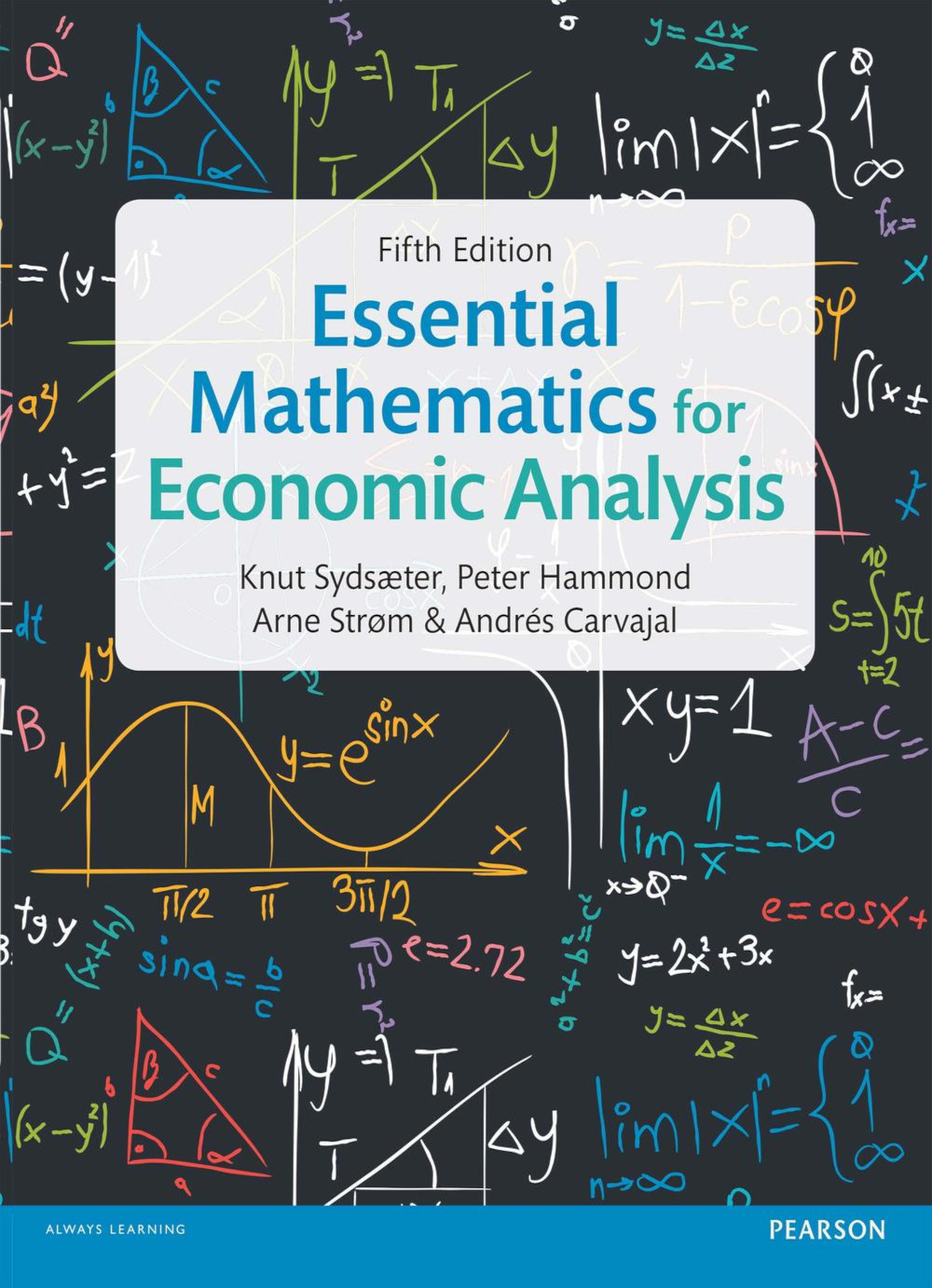
Venn diagram: union of two (overlapping) sets#
Relationships between sets can be visualized using Venn diagrams.
In this example, the red, brown and green areas are all part of \(A \cup B\): the union of set \(A\) (the left circle) and set \(B\) (the right circle).
Show code cell source
from matplotlib import pyplot as plt
from matplotlib_venn import venn2, venn2_circles

v = venn2(subsets=(1, 1, 1))
v.get_label_by_id('10').set_text('')
v.get_label_by_id('01').set_text('')
v.get_label_by_id('11').set_text('')

c = venn2_circles(subsets=(1, 1, 1), linestyle = 'solid')

# Style options
plt.title("Union of two overlapping sets")

# Add bracket showing the union of the two sets
plt.annotate('A ∪ B', xy=(0.5, 0), xytext=(0.5, -0.1), xycoords='axes fraction',
            fontsize=16, ha='center', va='top',
            bbox=dict(boxstyle='square', fc='white', color='k'),
            arrowprops=dict(arrowstyle='-[, widthB=9.5, lengthB=0.5', lw=2.0, color='k'))

plt.show()
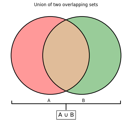
Venn diagram: intersection of two overlapping sets#
The intersection of the two sets, \(A \cap B\), is the brown area.
Show code cell source
from matplotlib import pyplot as plt
from matplotlib_venn import venn2, venn2_circles

v = venn2(subsets=(1, 1, 1))
v.get_label_by_id('10').set_text('')
v.get_label_by_id('01').set_text('')
v.get_label_by_id('11').set_text('$A \; ∩ \; B$')

c = venn2_circles(subsets=(1, 1, 1), linestyle = 'solid')

# Style options
plt.title("Intersection of two sets")

# Add legend
cols, texts = [],[]
cols.append(v.get_patch_by_id('11'))
texts.append(v.get_label_by_id('11')._text)
plt.legend(handles=cols, labels=texts, loc='upper right')

plt.show()
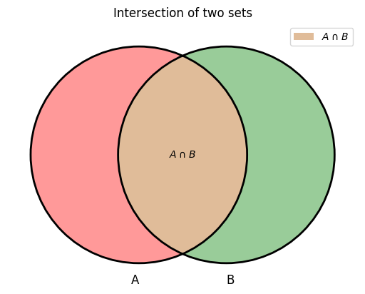
Venn diagram: intersection of two disjoint sets#
In this diagram, \(A\) and \(B\) are disjoint sets. Therefore, \(A \cap B = \varnothing\).
Show code cell source
from matplotlib import pyplot as plt
from matplotlib_venn import venn2, venn2_circles

v = venn2(subsets=(1, 1, 0))
v.get_label_by_id('10').set_text('')
v.get_label_by_id('01').set_text('')

c = venn2_circles(subsets=(1, 1, 0), linestyle = 'solid')

# Style options
plt.title("Intersection of disjoint sets is the empty set")

# Add legend
cols, texts = [],[]
for i in ('10', '01'):
    cols.append(v.get_patch_by_id(i))
    texts.append(v.get_label_by_id(i)._text)
# plt.legend(handles=cols, labels=texts)

plt.show()
Example
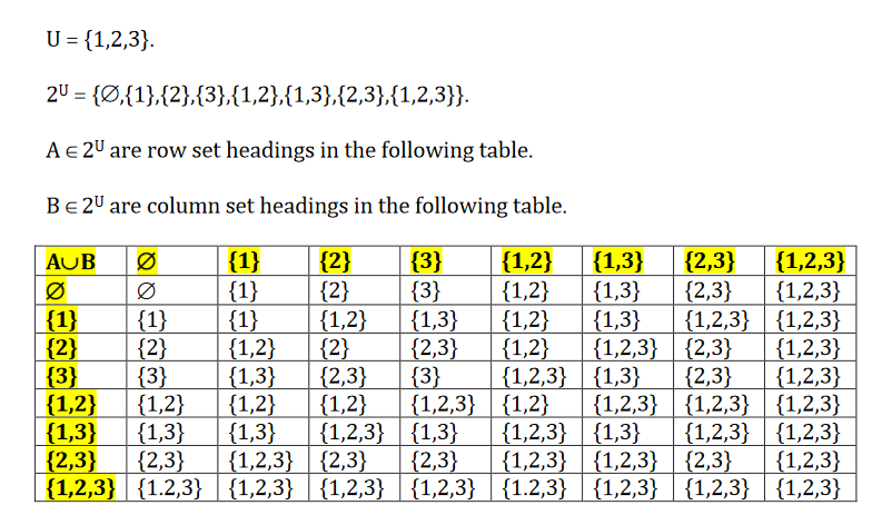
Fig. 1 Union example#
Example
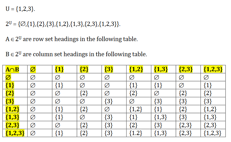
Fig. 2 Intersection example#
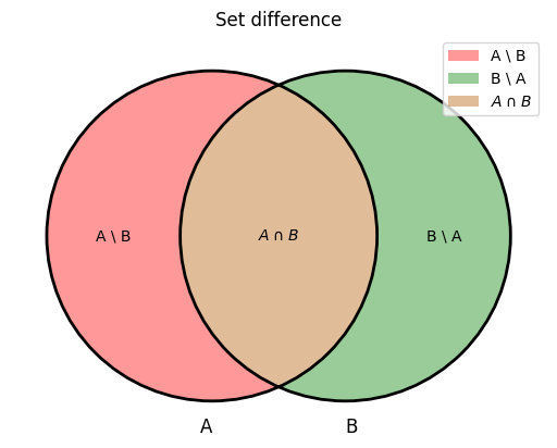
Exclusion and complementation#
Suppose that U is some universal set, \(X \subseteq U\) and \(Y \subseteq U\).
Definition
The set difference “X excluding Y”, which is denoted by \(X \setminus Y\), is the set
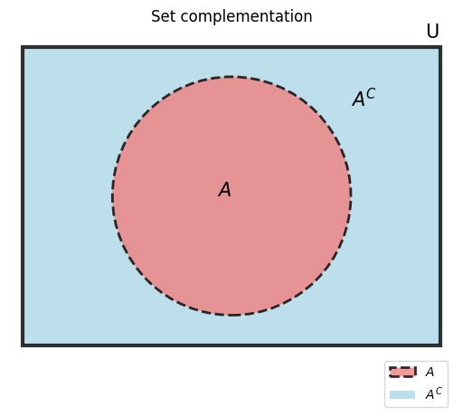
Definition
Set complementation is a special case of set exclusion. The complement of the set \(X\), which is denoted by \(X^C\) , is defined as \(X^C = U \setminus X\).
Note that \(X \cup X^C = U\) and \(X \cap X^C = \varnothing\).
Note
There are several alternative notations for the complement of a set, including \(X^C\), \(X'\), \(\bar{X}\), and \(\neg X\).
Venn diagram: set difference#
Show code cell source
from matplotlib import pyplot as plt
from matplotlib_venn import venn2, venn2_circles

v = venn2(subsets=(1, 1, 1))
v.get_label_by_id('10').set_text('A \\ B')
v.get_label_by_id('01').set_text('B \\ A')
v.get_label_by_id('11').set_text('$A \; ∩ \; B$')

c = venn2_circles(subsets=(1, 1, 1), linestyle = 'solid')

# Style options
plt.title("Set difference")

# Add legend
cols, texts = [],[]
for i in ('10', '01', '11'):
    cols.append(v.get_patch_by_id(i))
    texts.append(v.get_label_by_id(i)._text)
plt.legend(handles=cols, labels=texts, loc='upper right')

plt.show()
Venn diagram: set complementation#
Notice that the large rectangle containing both \(A\) and \(A^C\) is labelled \(U\), the universal set.
Show code cell source
from matplotlib import pyplot as plt
from matplotlib_venn import venn2, venn2_circles
from matplotlib.patches import Rectangle, Circle

fig, ax = plt.subplots()


ax.add_patch(Rectangle((-0.7, -0.5), 1.4, 1,
                       fc='lightblue',
                       alpha=0.8,
                       color='none',
                       linewidth=5))


ax.add_patch(Rectangle((-0.7, -0.5), 1.4, 1,
                       fc='none',
                       alpha=0.8,
                       color='black',
                       linewidth=3))


ax.add_patch(Circle((0, 0), 0.4,
                       fc='lightcoral',
                       alpha=0.8,
                       color='black',
                       linewidth=2,
                   linestyle='dashed'))

v = venn2(subsets=(1, 1, 1))
for i in ('10', '01', '11'):
    v.get_patch_by_id(i).set_alpha(0)
    v.get_label_by_id(i).set_text('')

v.get_label_by_id('A').set_text('')
v.get_label_by_id('B').set_text('')

# Style options
plt.title("Set complementation")

plt.text(0.65, 0.53, 'U', fontsize=15)
plt.text(-0.05, 0, '$A$', fontsize=15)
plt.text(0.4, 0.3, '$A^C$', fontsize=15)

cols, texts = [],[]
cols.append(ax.patches[2])
texts.append('$A$')
cols.append(ax.patches[0])
texts.append('$A^C$')

plt.legend(handles=cols, labels=texts, loc='lower right',
           bbox_to_anchor=(1, -0.15))


plt.show()
Example
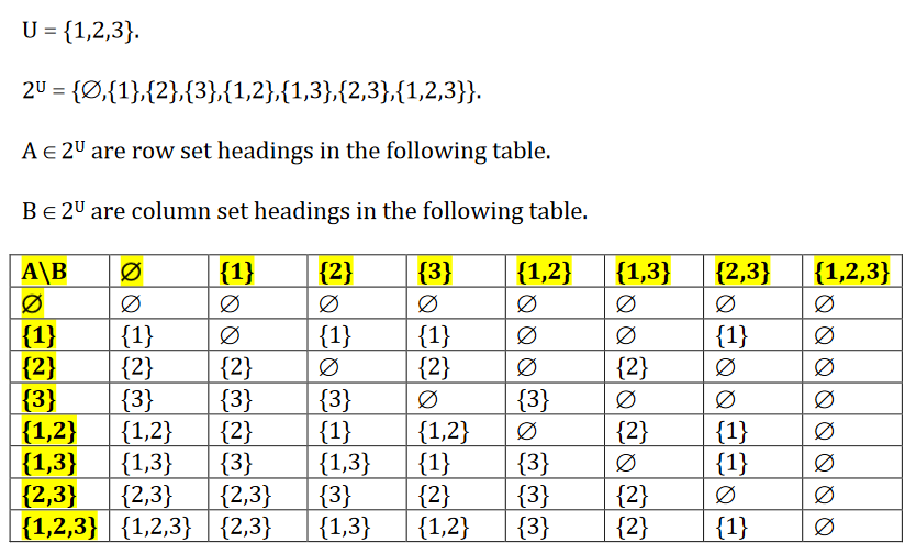
Fig. 3 Exclusion/set difference example#
Example: Set complement
Suppose that the universal set is \(U = \{1, 2, 3\}\). The power set for the set \(U\) in this example is
The elements of this power set are the subsets of the universal set. The complements for each of these subsets are:
\(\varnothing^C = U\)
\(\{1\}^C = \{2, 3\}\)
\(\{2\}^C = \{1, 3\}\)
\(\{3\}^C = \{1, 2\}\)
\(\{1, 2\}^C = \{3\}\)
\(\{1, 3\}^C = \{2\}\)
\(\{2, 3\}^C = \{1\}\)
\(U^C = \varnothing\)
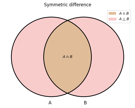
Symmetric difference#
Definition
The symmetric difference of \(X\) and \(Y\), which is denoted by \(X \bigtriangleup Y\), is the set
It is interesting to compare the operations of union and symmetric difference. They relate to alternative interpretions of the phrase “belongs to either \(X\) or \(Y\)”.
The set \(X \cup Y\) consists of all elements that are either in set \(X\) only, or in set \(Y\) only, or in both of these sets.
The set \(X \bigtriangleup Y\) consists of all elements that are either in set \(X\) only, or in set \(Y\) only, but are not in both of these sets.
Note
Exclusive or is another name for the symmetric difference operation.
Venn diagram: symmetric difference#
Note that the areas in light red together comprise the symmetric difference.
Show code cell source
from matplotlib import pyplot as plt
from matplotlib_venn import venn2, venn2_circles

v = venn2(subsets=(1, 1, 1))
v.get_label_by_id('10').set_text('')
v.get_label_by_id('01').set_text('')
v.get_label_by_id('11').set_text('$A \; ∩ \; B$')

v.get_patch_by_id('01').set_color('lightcoral')
v.get_patch_by_id('10').set_color('lightcoral')


c = venn2_circles(subsets=(1, 1, 1), linestyle = 'solid')

# Style options
plt.title("Symmetric difference")

# Add legend
cols, texts = [],[]
cols.append(v.get_patch_by_id('11'))
texts.append(v.get_label_by_id('11')._text)
cols.append(v.get_patch_by_id('10'))
texts.append('$A \; △ \; B$')
plt.legend(handles=cols, labels=texts, loc='upper right')

plt.show()
Example
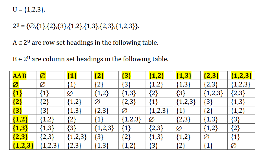
Fig. 4 Symmetric difference example#
De Morgan’s laws#
De Morgan’s law simple version
Suppose that \(X\) is some set, \(A \subseteq X\) and \(B \subseteq X\). According to De Morgan’s laws, we have
and
De Morgan’s law general version
Let \(I\) be some index set. Note that while I is allowed to be finite, it does not have to be finite. Let \(X\) be some set and suppose that \(A_i \subseteq U\) for all \(i \in I\). According to De Morgan’s laws, we have
and
Example
Let \(X = \{1, 2, 3\}, A = \{1, 2\} \subset X\) and \(B = \{2, 3\} \subset X\). Note that \(A \cup B = \{1, 2, 3\} = X\) and \(A \cap B = \{2\}\). Note also that
\(X \setminus A = \{3\}, X \setminus B = \{1\}\),
\(X \setminus (A \cup B) = X \setminus X = \varnothing\) and
\(X \setminus (A \cap B) = X \setminus \{2\} = \{1, 3\}\).
We have
and
The real number system#
There are several approaches for defining rigorously what numbers are:
axiomatic approach (real numbers are something that )
model-theoretic approach (Dedekind cuts)
The system of real numbers is an algebraic structure known as a complete ordered field. Indeed, in a sense, it is the only complete ordered field in existence. Any other complete ordered field turns out to be “isomoporhic” to the real number system. (The term “isomorphic” is a mathematical version of “essentially the same”).
The system of real numbers is formally denoted by \((\mathbb{R}, \mathbb{R}_{++}, +, \times)\), where \(+\) and \(\times\) are the familiar addition and multiplication operations for real numbers.
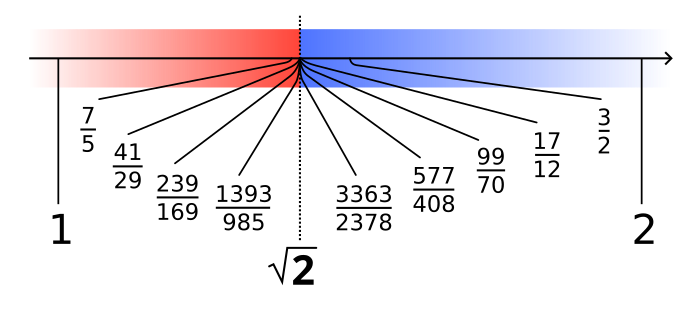
The set of real numbers \(\mathbb{R}\) can be viewed as the completion of the set of rational numbers \(\mathbb{Q}\) because it involves filling in the “holes” that exist in the set of rational numbers. These holes take the form of irrational numbers like \(\sqrt{2}\), \(\pi\) and \(e\).
Why aren’t the rationals enough?#
Why aren’t the rational numbers enough? What makes us think that they contain “holes”? This is a very good question. Especially when you realise that any numerical calculation on a computer will only generate a rational number.
A geometric argument for the existence of irrational numbers is perhaps the easiest way to convince yourself of their existence. Think about a right-angled triangle with a base (horizontal side) that is one metre long and whose (perpendicular) height (which is also its vertical side) is also one metre long. We know from Pythagoras’ Theorem that the length of the hypotenuse for this triangle is “the square root of two” metres long. But it can be shown that \(\sqrt{2}\) is an irrational number!
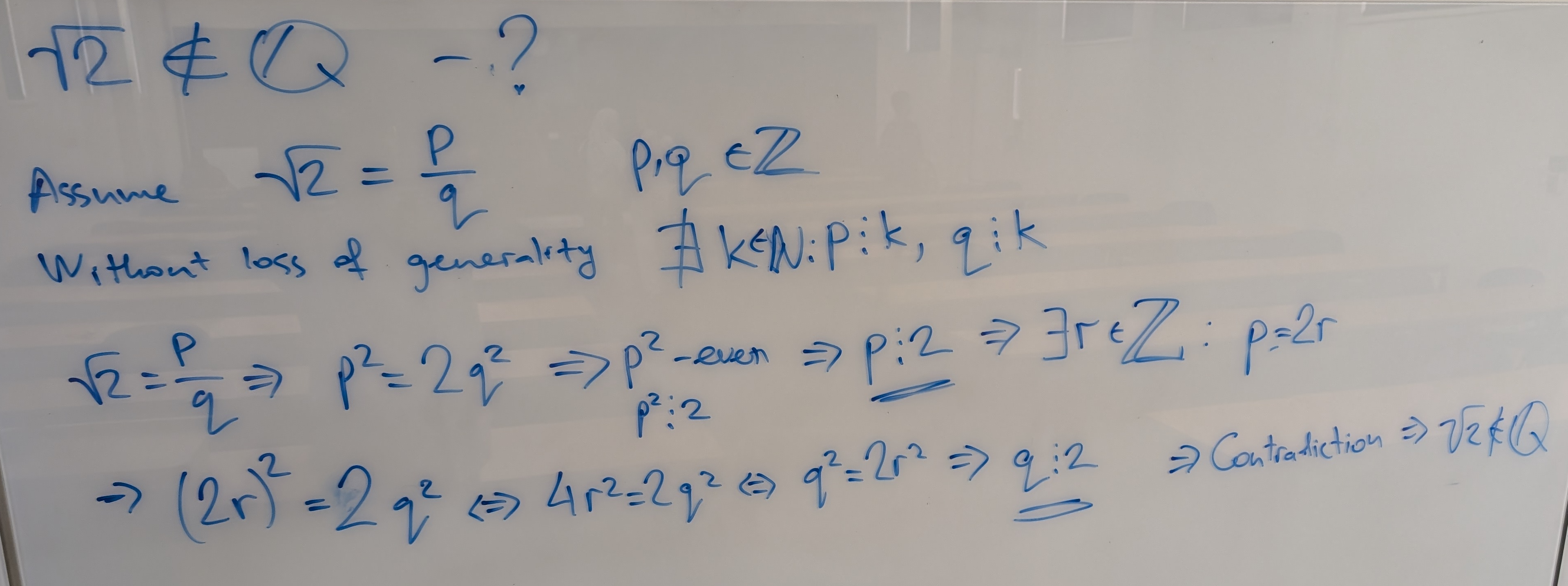
Proposition
\(\sqrt{2}\) is not a rational number.
Proof
We can prove this proposition by contradiction.
Assume that \(\sqrt{2} = \frac{p}{q}\) where \(p\) ad \(q\) are whole numbers.
Without loss of generality we can choose \(p\) and \(q\) such that they do not have common factors, otherwise these factors can be cancelled out.
Then \(\frac{p^2}{q^2} = 2\), and so \(2q^2 = p^2 \iff p^2\) is a multiple of 2.
All components in prime decomposition of \(p^2\) enter in pairs because it is a square, therefore there must be an even number of 2’s in the factorization of \(p^2\) \(\implies\) \(p\) is a multiple of 2 itself.
Therefore we can find a whole number \(r\) such that \(p = 2r\), and substitute to get \(2q^2 = 4r^2 \implies q^2 = 2r^2\).
Now the same arguments applied to \(q\) let us conclude that \(q\) is also a multiple of 2.
This contradicts our choice of \(p\) and \(q\) not having common factors!
Therefore our assumption that \(\sqrt{2} = \frac{p}{q}\) is false, and thus \(\sqrt{2}\) is indeed an irrational number. \(\blacksquare\)
Dedekind cuts and the density of set of rational numbers#
theoretical model of real numbers
allows for rigorous definition of real numbers in a constructive way without relying on the axioms
associates a real number to a set (rather, two sets forming a partition of another set)
Definition
A Dedekind cut is a partition of the rational numbers into two non-empty sets \(A\) and \(A'\) such that
every rational number is in either \(A\) or \(A'\), but not in both
every element of \(A\) is less than every element of \(A'\)
The set \(A\) is referred to as lower half, the set \(A'\) as upper half.
Examples of Dedekind cuts
\(A \subset \mathbb{Q}: \forall a \in A \:\: a < 1\), \(A' \subset \mathbb{Q}: \forall a' \in A' \:\: a' \ge 1\)
\(A \subset \mathbb{Q}: \forall a \in A \:\: a \le 1\), \(A' \subset \mathbb{Q}: \forall a' \in A' \:\: a' > 1\)
\(A \subset \mathbb{Q}: \forall a \in A \:\: a^2 < 2\), \(A' \subset \mathbb{Q}: \forall a' \in A' \:\: a'^2 > 2\)
Fact
The above three examples cover all possible cases for Dedekind cuts:
Upper half has the least element
Lower half has the greatest element
Neither half has the least or the greatest element
Proof
It is easy to show that it is impossible that both \(A\) has the greatest and \(A'\) has the least element. If it was possible, than there would be a rational number at midpoint between these two elements which would not belong to either \(A\) and \(A'\), which is a contradiction.
Let’s prove the third example case, namely that \(A\) has no greatest element (the absence of least element in \(A'\) is proven analogously). Consider any \(a \in A\), we have \(a^2<2\). We can show that there exists a natural number \(n \in \mathbb{N}\) such that
and therefore \(a+1/n \in A\). Indeed, the last inequality is equivalent to
The last inequality holds true if we impose \(\tfrac{2a+1}{n} < 2 - a^2\), therefore choosing \(n\) to satisfy
ensures that \(a + 1/n \in A\).
Thus, for any \(a \in A\) we can find a greater element \(a + 1/n \in A\), and therefore \(A\) has no greatest element. \(\blacksquare\)
Fact
Dedekind cut of the third type (those which do not have the least element in the upper half and the greatest element in the lower half) defines an irrational number.
irrational numbers are objects of new type, they are not rational numbers by construction
fill in the “holes” between rational numbers
rational numbers \(\mathbb{Q}\) and irrational numbers defined by Dedekind cuts form the set of real numbers \(\mathbb{R}\)
Fact
For any real numbers \(a,b \in \mathbb{R}\) where \(a>b\) there is a real number \(c \in \mathbb{R}\) such that \(b<c<a\).
Proof
Denote \(A|A'\) and \(B|B'\) the Dedekind cuts corresponding to \(a\) and \(b\) respectively.
Because \(a>b\), we have \(B \subset A\) yet \(B \ne A\). Thus, there exists a rational number \(c \in A \setminus B\).
We have \(c \in A\), that is \(c<a\). But \(c \notin B\), it follows that \(c \in B'\), and therefore \(c>b\)
Thus, \(b<c<a\). \(\blacksquare\)
it follows from the proof that the number \(c\) is in fact rational
it also follows by repeated application of the proposition that an infinite number of rational numbers can be fitted between any two given rational numbers, however close they are in the number line
overall, the number line of real numbers has no gaps!
What’s next?#
Same steps as in axiomatic approach to define the common sense operations, but using Dedekind cuts as the definition of real numbers.
rigorous definitions of number representation using Dedekind cuts
decimal representation
continued fractions
rigorous definitions of algebraic operations using Dedekind cuts
addition
subtraction
multiplication
division
rigorous definitions of order relations from set theory
less than
greater than
less than or equal to
greater than or equal to
rigorous definitions of convergence and limits
etc.
This is re-definition of all our “common sense” knowledge about numbers in a rigorous mathematical language \(\implies\) we can use standard arithmetic operations at a deeper level of mathematical rigour.
Example
Note
Division by zero in not defined for any real number \(p\).
Note
When exponent is fractional and base is negative, the result is undefined for non-integer exponents.
See discussion here
Counting elements in sets#
Definition
The number of elements of finite set \(X\) is called the cardinality of \(X\), and is denoted by any of the following notation:
\(\lvert X \rvert\)
\(\# X\)
\(nX\)
\(n(X)\)
Counting the number of a union or an intersection of two sets \(A\) and \(B\) applying common sense may be dangerous.
Example
What is the number of elements of \(A \cup B\), \(|A \cup B|\)?
But!
It depends on whether \(A\) and \(B\) are disjoint or not!
General rule
Therefore, \(|A \cup B| = |A| + |B|\) if and only if \(A \cap B = \emptyset\)
Note
Be careful when solving the problems involving cardinality!
Counting Cartesian Products#
Fact
If \(A_n\) are finite for \(n=1, \ldots,N\), then
That is, number of possible tuples \(=\) product of the number of possibilities for each element
Example
Number of binary sequences of length \(10\) is
Examples of sets in economics#
Some sets that you might encounter during your study of economics include:
Budget sets
Weak preference sets
Indifference sets
Input requirement sets
Isoquants
Isocosts
Price simplices (simplexes)
We will briefly consider some of these examples below.
Sigma notation
Sigma notation is used to quickly write sums of elements index by \(i\)
Sigma notation can be used with other operations as well, for example \(\prod_{i=1}^{n} A_i\) denotes a product, \(\times_{i=1}^{n} A_i\) denotes a Cartesian product, \(\cup_{i=1}^{n} A_i\) denotes a inion and \(\cap_{i=1}^{n} A_i\) denotes an intersection of \(A_i,\;\forall i\in\{1,\dots,n\}\).
Budget sets#
Linear prices with an income endowment:
Linear prices with a commodity bundle endowment:
These are examples of “lower contour sets” for expenditure by an individual.
Weak preference sets#
Reference commodity bundle version:
Reference utility level version:
These are examples of “(weak) upper contour sets” for the utility level attained by an individual.
Indifference sets#
Reference commodity bundle version:
Reference utility level version:
These are examples of “level sets” for the utility level attained by an individual.
Input requirement sets#
Consider a single output, multiple input production technology that can be represented by a production function of the form
An input requirement set for this production technology takes the form
This is an example of a “(weak) upper contour set” for the output level attained by a producer.
Isoquants#
Consider a single output, multiple input production technology that can be represented by a production function of the form
An isoquant for this production technology takes the form
This is an example of a “level set” or the output level attained by a producer.
Isocosts#
An isocost depicts the locus of all input combinations that cost the producer the same amount of money to employ.
Suppose that there are \(n \in \mathbb{N}\) distinct production inputs (or factors of production, if you prefer). An isocost for this situation takes the form
where \(w_i\) is the per-unit price of input \(i\).
This is an example of a “level set” for the expenditure on inputs by a producer.
Price simplex#
In some situations in economics, it is relative prices that matter, rather than the absolute level of each individual price. In such cases, some form of price normalisation can be employed.
Common normalisations involve choosing either a particular commodity, or a particular basket of commodities, to be the numeraire. The expenditure on the the numeraire commodity, or numeraire basket of commodities, is then set equal to one.
If the numeraire basket consists of one unit of each of the \(n\) final commodities in an economy, then the set of possible prices is given by:
This set is known as a price “simplex”.