📖 Limit of a function

📖 Limit of a function#

⏱ | words

Consider a univariate function $f: \mathbb{R} \rightarrow \mathbb{R}$ written as $f(x)$

The domain of $f$ is $\mathbb{R}$, the range of $f$ is a (possibly improper) subset of $\mathbb{R}$

[Spivak, 2006] (p. 90) provides the following informal definition of a limit: “The function $f$ approaches the limit $l$ near [the point $x =$] $a$, if we can make $f(x)$ as close as we like to $l$ by requiring that $x$ be sufficiently close to, but unequal to, $a$.”

Definition

The function $f: \mathbb{R} \rightarrow \mathbb{R}$ approaches the limit $l$ near [the point $x = a$] if for every $\epsilon > 0$, there is some $\delta > 0$ such that, for all $x$ such as $0 < |x − a| < \delta$, $|f(x) − l | < \epsilon$.

The absolute value $|\cdot|$ in this definition plays the role of general distance function $\|\cdot\|$ which would be appropriate for the functions from $\mathbb{R}^n$ to $\mathbb{R}^k$. We will also use $d(x,a)$ to denote distance, i.e. $d(x,a) = |x-a|$ in multivariate cases later in the course.

Suppose that the limit of $f$ as $x$ approaches $a$ is $l$. We can write this as

\[ \lim_{x \rightarrow a} f(x) = l \]

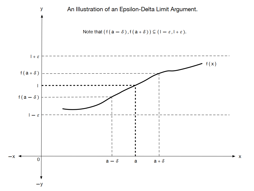
_images/epsilon_delta.png — Fig. 24 An illustration of an epsilon-delta limit argument#

The structure of $\epsilon–\delta$ arguments#

Suppose that we want to attempt to show that $\lim _{x \rightarrow a} f(x)=b$.

In order to do this, we need to show that, for any choice $\epsilon>0$, there exists some $\delta_{\epsilon}>0$ such that, whenever $|x-a|<\delta_{\epsilon}$, it is the case that $|f(x)-b|<\epsilon$.

We write $\delta_{\epsilon}$ to indicate that the choice of $\delta$ is allowed to vary with the choice of $\epsilon$.

An often fruitful approach to the construction of a formal $\epsilon$-$\delta$ limit argument is to proceed as follows:

Start with the end-point that we need to establish: $|f(x)-b|<\epsilon$.
Use appropriate algebraic rules to rearrange this “final” inequality into something of the form $|k(x)(x-a)|<\epsilon$.
This new version of the required inequality can be rewritten as $|k(x)||(x-a)|<\epsilon$.
If $k(x)=k$, a constant that does not vary with $x$, then this inequality becomes $|k||x-a|<\epsilon$. In such cases, we must have $|x-a|<\frac{\epsilon}{|k|}$, so that an appropriate choice of $\delta_{\epsilon}$ is $\delta_{\epsilon}=\frac{\epsilon}{|k|}$.
If $k(x)$ does vary with $x$, then we have to work a little bit harder.

Suppose that $k(x)$ does vary with $x$. How might we proceed in that case? One possibility is to see if we can find a restriction on the range of values for $\delta$ that we consider that will allow us to place an upper bound on the value taken by $|k(x)|$.

In other words, we try and find some restriction on $\delta$ that will ensure that $|k(x)|<K$ for some finite $K>0$. The type of restriction on the values of $\delta$ that you choose would ideally look something like $\delta<D$, for some fixed real number $D>0$. (The reason for this is that it is typically small deviations of $x$ from a that will cause us problems rather than large deviations of $x$ from a.)

If $0<|k(x)|<K$ whenever $0<\delta<D$, then we have

\[ |k(x)||x-a|<\epsilon \Longleftarrow K|x-a|<\epsilon \Longleftrightarrow|x-a|<\frac{\epsilon}{K} . \]

In such cases, an appropriate choice of $\delta_{\epsilon}$ is $\delta_{\epsilon}=\min \left\{\frac{\epsilon}{K}, D\right\}$.

Example

Consider the mapping $f: \mathbb{R} \longrightarrow \mathbb{R}$ defined by $f(x)=7 x-4$.

We want to show that $\lim _{x \rightarrow 2} f(x)=10$.

Note that $|f(x)-10|=|7 x-4-10|=|7 x-14|=|7(x-2)|=$ $|7||x-2|=7|x-2|$.
We require $|f(x)-10|<\epsilon$, but:

\[ |f(x)-10|<\epsilon \Longleftrightarrow 7|x-2|<\epsilon \Longleftrightarrow|x-2|<\frac{\epsilon}{7} \]

Thus, for any $\epsilon>0$, if $\delta_{\epsilon}=\frac{\epsilon}{7}$, then $|f(x)-10|<\epsilon$ whenever $|x-2|<\delta_{\epsilon}$.

Example

Consider the mapping $f: \mathbb{R} \longrightarrow \mathbb{R}$ defined by $f(x)=x^{2}$

We want to show that $\lim _{x \rightarrow 2} f(x)=4$.

Note that $|f(x)-4|=\left|x^{2}-4\right|=|(x+2)(x-2)|=|x+2||x-2|$.
Suppose that $|x-2|<\delta$, which in turn means that $(2-\delta)<x<(2+\delta)$. Thus we have $(4-\delta)<(x+2)<(4+\delta)$.
Let us restrict attention to $\delta \in(0,1)$. This gives us $3<(x+2)<5$, so that $|x+2|<5$.
Thus, when $|x-2|<\delta$ and $\delta \in(0,1)$, we have $|f(x)-4|=|x+2||x-2|<5 \delta$.
We require $|f(x)-4|<\epsilon$. One way to ensure this is to set $\delta_{\epsilon}=\min \left(1, \frac{\epsilon}{5}\right)$.

Example

Consider the mapping $f: \mathbb{R} \rightarrow \mathbb{R}$ defined by $f(x) = x^2 − 3x + 1$.

We want to show that $\lim_{x \rightarrow 2} f(x ) = −1$.

Note that $|f(x) − (−1)| = |x^2 − 3x + 1 + 1| = |x^2 − 3x + 2|$ $= |(x − 1)(x − 2)| = |x − 1||x − 2|$.
Suppose that $|x − 2| < \delta$, which in turn means that $(2 − \delta) < x < (2 + \delta)$. Thus we have $(1 − \delta) < (x − 1) < (1 + \delta)$.
Let us restrict attention to $\delta \in (0, 1)$. This gives us $0 < (x − 1) < 2$, so that $|x − 1| < 2$.
Thus, when $|x − 2| < \delta$ and $\delta \in (0, 1)$, we have $|f(x) − (−1)| = |x − 1||x − 2| < 2\delta$.
We require $|f(x) − (−1)| < \epsilon$. One way to ensure this is to set $\delta_\epsilon = \min(1, \frac{\epsilon}{2} )$.

The above examples are drawn from Willis Lauritz Peterson of the University of Utah

A useful fact in these derivations is also

Fact

For any $a, b \in \mathbb{R}$ which have opposite signs $ab<0$ it holds that

\[ a \leqslant x \leqslant b, \; ab<0 \quad \impliedby \quad |x| \leqslant \min(|a|, |b|) \]

Proof

Draw a picture, careful with implication direction!

Example

Consider the mapping $f: \mathbb{R} \rightarrow \mathbb{R}$ defined by $f(x) = \exp(x-1)$.

We want to show that $\lim_{x \rightarrow 2} f(x) = e$

We need to ensure that for any $\epsilon>0$ it holds that $|f(x) − e| < \epsilon$, i.e. $|\exp(x-1) − e| < \epsilon$

\[\begin{split} |\exp(x-1) − e| < \epsilon \\ - \epsilon < \exp(x-1) -e < \epsilon \\ e - \epsilon < \exp(x-1) < e+\epsilon \\ \ln(e - \epsilon) < x-1 < \ln(e+\epsilon) \\ \ln(e - \epsilon)-1 < x-2 < \ln(e+\epsilon)-1 \end{split}\]

It is clear that $\ln(e)-1 = 0$, therefore $\ln(e-\epsilon)-1 < 0$, and similarly $\ln(e+\epsilon)-1 > 0$. Therefore

\[\begin{split} |x-2| <& \min\{ |\ln(e-\epsilon)-1|,|\ln(e+\epsilon)-1|\} \\ &= \min\{ 1-\ln(e-\epsilon),\ln(e+\epsilon)-1\} \end{split}\]

Thus, taking $\delta = \min\{ 1-\ln(e-\epsilon),\ln(e+\epsilon)-1\}$ ensures the required inequality.

We can further simplify by analyzing the minimum itself to conclude that it is attained at $1-\ln(e-\epsilon)$.

Heine and Cauchy definitions of the limit for functions#

As a side note, let’s mention that there are two ways to define the limit of a function $f$.

The above $\epsilon$-$\delta$ definition is is due to Augustin-Louis Cauchy.

The limit for functions can also be defined through the limit of sequences we were talking about in the last lecture. This equivalent definition is due to Eduard Heine

Definition (Limit of a function due to Heine)

Given the function $f: A \subset \mathbb{R} \to \mathbb{R}$, $a \in \mathbb{R}$ is a limit of $f(x)$ as $x \to x_0 \in A$ if

\[\forall \{x_n\} \in A \colon \lim_{n \to \infty} x_n = x_0 \in A \quad \implies \quad f(x_n) \to a \;\text{as}\; n \to \infty\]

note the crucial requirement that $f(x_n) \to a$ has to hold for all converging to $x_0$ sequences $\{x_n\}$ in $A$
note also how the Cauchy definition is similar to the definition of a limit to a sequence

Fact

Cauchy and Heine definitions of the function limit are equivalent

Therefore we can use the same notation of the definition of the limit of a function

\[\lim_{x \to x_0} f(x) = a \quad \text{or} \quad f(x) \to a \; \text{as} \; x \to x_0\]

Properties of the limits#

In practice, we would like to be able to find at least some limits without having to resort to the formal “epsilon-delta” arguments that define them. The following rules can sometimes assist us with this.

Fact

Let $c \in \mathbb{R}$ be a fixed constant, $a \in \mathbb{R}, \alpha \in \mathbb{R}, \beta \in \mathbb{R}, n \in \mathbb{N}$, $f: \mathbb{R} \longrightarrow \mathbb{R}$ be a function for which $\lim _{x \rightarrow a} f(x)=\alpha$, and $g: \mathbb{R} \longrightarrow \mathbb{R}$ be a function for which $\lim _{x \rightarrow a} g(x)=\beta$. The following rules apply for limits:

$\lim _{x \rightarrow a} c=c$ for any $a \in \mathbb{R}$.
$\lim _{x \rightarrow a}(c f(x))=c\left(\lim _{x \rightarrow a} f(x)\right)=c \alpha$.
$\lim _{x \rightarrow a}(f(x)+g(x))=\left(\lim _{x \rightarrow a} f(x)\right)+\left(\lim _{x \rightarrow a} g(x)\right)=\alpha+\beta$.
$\lim _{x \rightarrow a}(f(x) g(x))=\left(\lim _{x \rightarrow a} f(x)\right)\left(\lim _{x \rightarrow a} g(x)\right)=\alpha \beta$.
$\lim _{x \rightarrow a}\left(\frac{f(x)}{g(x)}\right)=\frac{\lim _{x \rightarrow a} f(x)}{\lim _{x \rightarrow a} g(x)}=\frac{\alpha}{\beta}$ whenever $\beta \neq 0$.
$\lim _{x \rightarrow a} \sqrt[n]{f(x)}=\sqrt[n]{\lim _{x \rightarrow a} f(x)}=\sqrt[n]{\alpha}$ whenever $\sqrt[n]{\alpha}$ is defined.
$\lim _{x \rightarrow a} \ln f(x)=\ln \lim _{x \rightarrow a} f(x)=\ln \alpha$ whenever $\ln \alpha$ is defined.
$\lim _{x \rightarrow a} e^{f(x)}=\exp\big(\lim _{x \rightarrow a} f(x)\big)=e^{\alpha}$
After we have learned about differentiation, we will learn about another useful rule for limits that is known as “L’Hopital’s rule”.

Fact

Weak inequalities are preserved in the limit. Consider two functions $f: \mathbb{R} \to \mathbb{R}$ and $g: \mathbb{R} \to \mathbb{R}$, when limits with $x \to x_0$ exist, it holds that

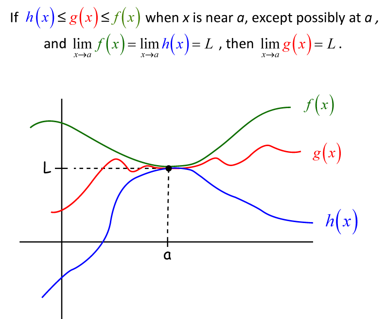
\[ f(x) \geqslant g(x) \;\text{for all}\;x \in \mathbb{R}\setminus\{x_0\},\; \quad \implies \lim_{x \to x_0} f(x) \geqslant \lim_{x \to x_0} g(x) \]

\[ f(x) > g(x) \;\text{for all}\;x\in \mathbb{R}\setminus\{x_0\},\; \quad \implies \lim_{x \to x_0} f(x) \geqslant \lim_{x \to x_0} g(x) \]

Fact (Squeeze theorem)

Consider three functions $f: \mathbb{R} \to \mathbb{R}$, $g: \mathbb{R} \to \mathbb{R}$ and $h: \mathbb{R} \to \mathbb{R}$. If

\[ f(x) \geqslant g(x) \geqslant h(x) \;\text{for all} \;x\in \mathbb{R}\setminus\{x_0\}, \]

\[ \lim_{x \to x_0} f(x) = \lim_{x \to x_0} h(x) = L, \]

then $\lim_{x \to x_0} g(x) = L$.

statement both about existence of the limit for $g(x)$ as $x \to x_0$
and about the value of this limit

Example

Limits can sometimes exist even when the function being considered is not so well behaved. One such example is provided by [Spivak, 2006] (pp. 91–92). It involves the use of a trigonometric function.

The example involves the function $f: \mathbb{R} \setminus 0 \rightarrow \mathbb{R}$ that is defined by $f(x) = x \sin ( \frac{1}{x})$.

Clearly this function is not defined when $x = 0$. Furthermore, it can be shown that $\lim_{x \rightarrow 0} \sin ( \frac{1}{x})$ does not exist. However, it can also be shown that $\lim_{x \rightarrow 0} f(x) = 0$.

The reason for this is that $\sin (\theta) \in [−1, 1]$ for all $\theta \in \mathbb{R}$. Thus $\sin ( \frac{1}{x} )$ is bounded above and below by finite numbers as $x \rightarrow 0$. This allows the $x$ component of $x \sin (\frac{1}{x})$ to dominate as $x \rightarrow 0$.

Formally, we can use the squeeze theorem noting that $-1 \leqslant \sim(1/x) \leqslant 1$. We can write the following double inequality and take limits on the left and right sides as $x \to 0$:

\[\begin{split} \begin{array}{ccccc} -|x| &\leq& x \sin (\tfrac{1}{x}) &\leq& |x| \\ \downarrow &\leq& \downarrow &\leq& \downarrow \\ 0 &\leq& \lim_{x \to 0} x \sin (\tfrac{1}{x}) &\leq& 0 \end{array} \end{split}\]

Therefore by the squeeze theorem $\lim_{x \to 0} x \sin (\tfrac{1}{x}) = 0$.

Example

Limits do not always exist. In this example, we consider a case in which the limit of a function as $x$ approaches a particular point does not exist.

Consider the mapping $f: \mathbb{R} \rightarrow \mathbb{R}$ defined by

\[\begin{split} f(x ) = \begin{cases} 1 \quad \text{ if } x \geqslant 5; \\ 0 \quad \text{ if } x < 5 \end{cases} \end{split}\]

We want to show that $\lim_{x \rightarrow 5} f(x)$ does not exist.

Suppose that the limit does exist. Denote the limit by $l$. Let $\delta > 0$.

If $|5 − x | < \delta$, then $5 − \delta < x < 5 + \delta$, so that $x \in (5 − \delta, 5 + \delta) = (5 − \delta, 5) \cup [5, 5 + \delta)$, where $(5 − \delta, 5) \ne \varnothing$ and $[5, 5 + \delta) \ne \varnothing$.

Thus we know the following:

There exist some $x \in (5 − \delta, 5) \subseteq (5 − \delta, 5 + \delta)$, so that $f(x) = 0$ for some $x \in (5 − \delta, 5 + \delta)$.
There exist some $x \in [5, 5 + \delta) \subseteq (5 − \delta, 5 + \delta)$, so that $f(x) = 1$ for some $x \in (5 − \delta, 5 + \delta)$.
The image set under $f$ for the interval $(5 − \delta, 5 + \delta)$ is $f \big((5 − \delta, 5 + \delta)\big) = \{ f(x) : x \in (5 − \delta, 5 + \delta) \} = \{ 0, 1 \} \subseteq [0, 1]$.
Note that for any choice of $\delta > 0$, $[0, 1]$ is the smallest connected interval that contains the image set $f \big((5 − \delta, 5 + \delta)\big) = \{ 0, 1 \}$.

Hence, in order for the limit to exist, we need $[0, 1] \subseteq (l − \epsilon, l + \epsilon)$ for all $\epsilon > 0$. But for $\epsilon \in (0, \frac{1}{2})$, there is no $l \in \mathbb{R}$ for which this is the case. Thus we can conclude that $\lim_{x \rightarrow 5} f(x)$ does not exist.

Example

In the above example the limit definition by Heine is also useful for the proof.

Consider two sequences $\{x_n\}$ and $\{y_n\}$ such that $x_n \to 5$ and $y_n \to 5$. Let $x_n = 5 - 1/n$ and $y_n = 5+ 1/n$.

Function $f(x)$ computed at the values of $\{x_n\}$ forms a sequence of zeros which converges to $0$.
Function $f(x)$ computed at the values of $\{y_n\}$ forms a sequence of ones which converges to $1$.
Therefore, the limit of $f(x)$ does not exist.

Function continuity#

Our focus here is on continuous real-valued functions of a single real variable. In other words, functions of the form $f : X \rightarrow \mathbb{R}$ where $X \subseteq \mathbb{R}$.

Before looking at the picky technical details of the concept of continuity, it is worth thinking about that concept intuitively. Basically, a real-valued function of a single real-valued variable is continuous if you could potentially draw its graph without lifting your pen from the page. In other words, there are no holes in the graph of the function and there are no jumps in the graph of the function.

Definition

Let $f \colon A \to \mathbb{R}$

$f$ is called continuous at $a \in A$ if

\[\forall \{x_n\} \in A \colon \lim_{n \to \infty} x_n = a \in A \quad \implies \quad f(x_n) \to f(a) \]

Or, alternatively,

\[\lim_{x \to a} f(x) = f(a)\]

Definition

$f: A \to \mathbb{R}$ is called continuous if it is continuous at every $x \in A$

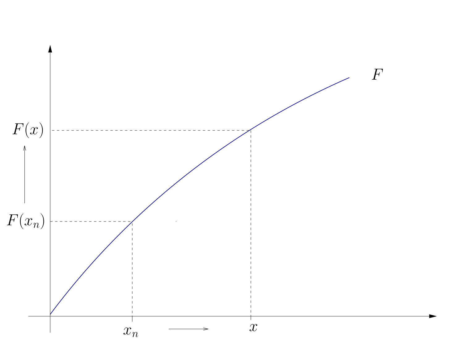
_images/cont_func.png — Fig. 25 Continuous function#

Example

Function $f(x) = \exp(x)$ is continuous at $x=0$

Proof:

Consider any sequence $\{x_n\}$ which converges to $0$

We want to show that for any $\epsilon>0$ there exists $N$ such that $n \geq N \implies |f(x_n) - f(0)| < \epsilon$. We have

\[\begin{split}\begin{array}{l} |f(x_n) - f(0)| = |\exp(x_n) - 1| < \epsilon \quad \iff \\ \exp(x_n) - 1 < \epsilon \; \text{ and } \; \exp(x_n) - 1 > -\epsilon \quad \iff \\ x_n < \ln(1+\epsilon) \; \text{ and } \; x_n > \ln(1-\epsilon) \quad \Longleftarrow \\ | x_n - 0 | < \min \big(\ln(1+\epsilon),\ln(1-\epsilon) \big) = \ln(1-\epsilon) \end{array}\end{split}\]

Because due to $x_n \to x$ for any $\epsilon' = \ln(1-\epsilon)$ there exists $N$ such that $n \geq N \implies |x_n - 0| < \epsilon'$, we have $f(x_n) \to f(x)$ by definition. Thus, $f$ is continuous at $x=0$.

Fact

Some functions known to be continuous on their domains:

$f: x \mapsto x^\alpha$
$f: x \mapsto |x|$
$f: x \mapsto \log(x)$
$f: x \mapsto \exp(x)$
$f: x \mapsto \sin(x)$
$f: x \mapsto \cos(x)$

Fact

Let $f$ and $g$ be functions and let $\alpha \in \mathbb{R}$

If $f$ and $g$ are continuous at $x$ then so is $f + g$, where

\[(f + g)(x) := f(x) + g(x)\]

If $f$ is continuous at $x$ then so is $\alpha f$, where

\[(\alpha f)(x) := \alpha f(x)\]

If $f$ and $g$ are continuous at $x$ then so is $f \cdot g$, where

\[(f \cdot g)(x) := f(x) \cdot g(x)\]

If $g(x) \ne 0$, $f$ and $g$ are continuous at $x$ then so is $f / g$, where

\[(f / g)(x) := f(x) / g(x)\]

If $f$ and $g$ are continuous at $x$ and real valued then so is $f \circ g$, where

\[(f \circ g)(x) := f( g(x))\]

Proof

Just repeatedly apply the properties of the limits

Let’s just check that

\[\text{$f$ and $g$ continuous at $x$} \implies \text{$f + g$ continuous at $x$}\]

Let $f$ and $g$ be continuous at $x$

Pick any $x_n \to x$

We claim that $f(x_n) + g(x_n) \to f(x) + g(x)$

By assumption, $f(x_n) \to f(x)$ and $g(x_n) \to g(x)$

From this and the triangle inequality we get

\[\| f(x_n) + g(x_n) - (f(x) + g(x)) \| \leqslant\]

\[\leqslant \| f(x_n) - f(x) \| + \| g(x_n) - g(x) \| \to 0\]

As a result, set of continuous functions is “closed” under elementary arithmetic operations

Example

The function $f \colon \mathbb{R} \to \mathbb{R}$ defined by

\[f(x) = \frac{\exp(x) + \sin(x)}{2 + \cos(x)} + \frac{x^4}{2} - \frac{\cos^3(x)}{8!}\]

is continuous (we just have to be careful to ensure that denominator is not zero – which it is not for all $x\in\mathbb{R}$)

Types of discontinuities#

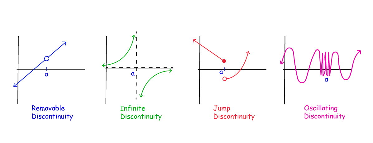
_images/4-types-of-discontinuity.png — Fig. 26 4 common types of discontinuity#

Example

The indicator function $x \mapsto \mathbb{1}\{x > 0\}$ has a jump discontinuity at $0$.

Example

An example of oscillating discontinuity is the function $f(x) = \sin(1/x)$ which is discontinuous at $x=0$.

Video to illustrate this function

Example

Consider the mapping $f : \mathbb{R} \rightarrow \mathbb{R}$ defined by $f(x ) = x^2$. We want to show that $f(x)$ is continuous at the point $x = 2$.

Note that $|f (2) − f(x)| = |f(x) − f (2)| = |x^2 − 4| = |x − 2||x + 2|$.

Suppose that $|2 − x | < \delta$. This means that $|x − 2| < \delta$, which in turn means that $(2 − \delta) < x < (2 + \delta)$. Thus we have $(4 − \delta) < (x + 2) < (4 + \delta)$.

Let us restrict attention to $\delta \in (0, 1)$. This gives us $3 < (x + 2) < 5$, so that $|x + 2| < 5$.

We have $|f (2) − f(x)| = |f(x) − f (2)| = |x − 2||x + 2| < (\delta)(5) = 5\delta$.

We require $|f (2) − f(x)| < \epsilon$. One way to ensure this is to set $\delta = \min(1, \frac{\epsilon}{5})$.

Example

Consider the mapping $f: \mathbb{R} \rightarrow \mathbb{R}$ defined by

\[\begin{split} f(x ) = \begin{cases} 1 \quad \text{ if } x > 5; \\ 0 \quad \text{ if } x < 5 \end{cases} \end{split}\]

We have already shown that $\lim_{x \rightarrow 5} f(x)$ does not exist. This means that it is impossible for $\lim_{x \rightarrow 5} f(x) = f (5)$. As such, we know that $f(x)$ is not continuous at the point $x = 5$.

This means that f(x) is not a continuous function.

However, it can be shown that (i) $f(x )$ is continuous on the interval $(−\infty, 5)$, and that (ii) $f(x)$ is continuous on the interval $(5, \infty)$. Why this is the case?

Example

Consider the mapping $f: \mathbb{R} \rightarrow \mathbb{R}$ defined by

\[\begin{split} f(x) = \begin{cases} \frac{1}{x} \quad \text{ if } x \ne 0; \\ 0 \quad \text{ if } x = 0. \end{cases} \end{split}\]

This function is a rectangular hyperbola when $x \ne 0$, but it takes on the value $0$ when $x = 0$. Recall that the rectangular hyperbola part of this function is not defined at the point $x = 0$.

This function is discontinuous at the point $x = 0$. Illustrate the graph of this function on the whiteboard.

Example

Consider the mapping $f: \mathbb{R} \rightarrow \mathbb{R}$ defined by

\[\begin{split} f(x) = \begin{cases} 1 \quad \text{ if } x \in Q; \\ 0 \quad \text{ if } x \notin Q \end{cases} \end{split}\]

This function is sometimes known as Dirichlet’s discontinuous function. It is discontinuous at every point in its domain.

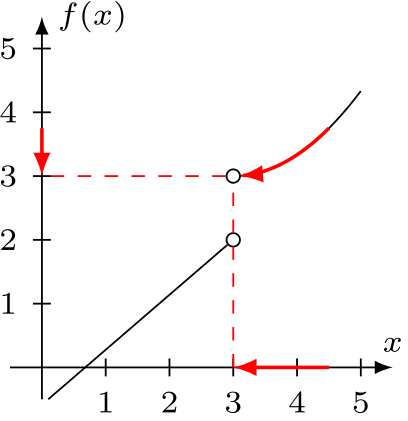
One-sided limits#

Definition

Given the function $f: A \subset \mathbb{R} \to \mathbb{R}$, $a \in \mathbb{R}$ is a limit from above of $f(x)$ as $x \to x_0^+ \in A$ if

\[\forall \{x_n\} \in A, x_n>x_0 \colon \lim_{n \to \infty} x_n = x_0 \in A \quad \implies \quad f(x_n) \to a \]

Notation for the limit from above is

\[ \lim_{x \to x_0^+} f(x) = a \]

Definition

Given the function $f: A \subset \mathbb{R} \to \mathbb{R}$, $a \in \mathbb{R}$ is a limit from below of $f(x)$ as $x \to x_0^- \in A$ if

\[\forall \{x_n\} \in A, x_n<x_0 \colon \lim_{n \to \infty} x_n = x_0 \in A \quad \implies \quad f(x_n) \to a \]

Notation for the limit from below is

\[ \lim_{x \to x_0^-} f(x) = a \]

Note

Compare to normal Heine limit definition

One-sided limits are useful for defining continuity of functions on closed intervals and in other situations

Fact

If $\lim_{x \to x_0} f(x) = a$ then $\lim_{x \to x_0^+} f(x) = \lim_{x \to x_0^-} f(x) = a$.

If $\lim_{x \to x_0^+} f(x) = \lim_{x \to x_0^-} f(x) = a$ then $\lim_{x \to x_0} f(x) = a$.

Proof

Proof is by careful definition of Heine limit and observing that the restrictions on the sequences in the one-sided limits are complementary. $\blacksquare$

When the two one-sided limits of a function take different values, the function has a jump discontinuity at that point

Fact

All properties of the limits hold for one-sided limits.

Limit at infinity#

Consider the logistic function (aka sigmoid)

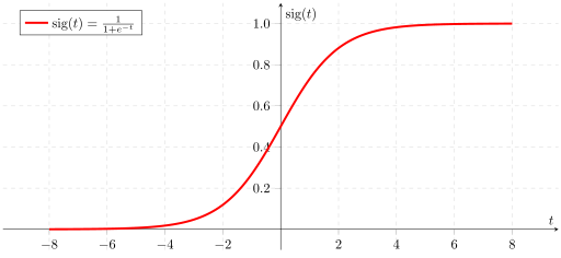
\[ f(x): \mathbb{R} \ni x \mapsto \frac{1}{1 + \exp(-x)} \in (0, 1) \subset \mathbb{R} \]

How to express the notion that the function approaches $1$ as $x$ goes to infinity?

Definition

The function $f: \mathbb{R} \rightarrow \mathbb{R}$ approaches the limit $l$ at infinity if for every $\epsilon > 0$, there is some $M > 0$ such that, for all $x$ such as $x > M$, $|f(x) − l | < \epsilon$.

Limit at infinity is denoted as

\[ \lim_{x \to \infty} f(x) = l \quad \text{or} \quad f(x) \to l \; \text{as} \; x \to \infty \]

Definition

The function $f: \mathbb{R} \rightarrow \mathbb{R}$ approaches the limit $l$ at negative infinity if for every $\epsilon > 0$, there is some $M < 0$ such that, for all $x$ such as $x < M$, $|f(x) − l | < \epsilon$.

Limit at negative infinity is denoted as

\[ \lim_{x \to -\infty} f(x) = l \quad \text{or} \quad f(x) \to l \; \text{as} \; x \to -\infty \]

Example

In statistics, the probability density functions have zero limit on infinity and negative infinity, and cumulative distribution functions have limits of 1 and 0 on infinity and negative infinity, respectively.

Fact

Limits at infinity support addition and multiplication rules for limits:

\[ \lim_{x \to \infty} (f(x) + g(x)) = \lim_{x \to \infty} f(x) + \lim_{x \to \infty} g(x) \]

\[ \lim_{x \to \infty} (f(x)g(x)) = \big(\lim_{x \to \infty} f(x)\big) \big( \lim_{x \to \infty} g(x)\big) \]

But not subtraction and division rules!

\[ \lim_{x \to \infty} (f(x) - g(x)) \neq \lim_{x \to \infty} f(x) - \lim_{x \to \infty} g(x) \]

\[ \lim_{x \to \infty} (f(x)/g(x)) \neq \big(\lim_{x \to \infty} f(x)\big) / \big( \lim_{x \to \infty} g(x)\big) \]

Example

\[ f(x) = x + 1, \quad g(x) = x \]

Now, compute their limits as $ x \to \infty $:

\[ \lim_{x \to \infty} f(x) = \lim_{x \to \infty} (x + 1) = \infty \]

\[ \lim_{x \to \infty} g(x) = \lim_{x \to \infty} x = \infty \]

The division of these functions is:

\[ \lim_{x \to \infty} \frac{f(x)}{g(x)} = \lim_{x \to \infty} \frac{x + 1}{x} \]

Simplifying,

\[ \lim_{x \to \infty} \left( 1 + \frac{1}{x} \right) = 1 + 0 = 1 \]

However, applying the division rule formally would suggest infinity over infinity which is an indeterminate form.

📖 Limit of a function

Contents

📖 Limit of a function#

The structure of \(\epsilon–\delta\) arguments#

Heine and Cauchy definitions of the limit for functions#

Properties of the limits#

Function continuity#

Types of discontinuities#

One-sided limits#

Limit at infinity#