📖 Functions and other mappings

⏱ | words

References and additional materials

[Sydsæter, Hammond, Strøm, and Carvajal, 2016]

Chapters 4.2, 4.3, 5.1 - 5.3

Mappings

Definition

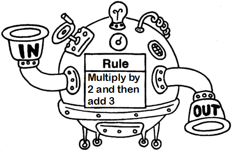
A generic mapping \(f\) from \(A\) to \(B\) is a rule that assigns elements \(x\) of a set \(A\) to elements of a set \(B\). We write

\[f: A \to B \qquad\text{ or }\qquad f: A \ni x \mapsto f(x) \in B\]

There are four basic types of mappings:

1. A one-to-one mapping:

   • \(\forall x \in X\) there is at most one \(f(x) \in Y\); and

   • \(\forall y \in Y\) there is at most one \(x \in X\) such that \(f(x)=y\).

   • example: \(f(x) = x\)

2. A many-to-one mapping:

   • \(\forall x \in X\) there is at most one \(f(x) \in Y\); but

   • \(\exists y \in Y\) for which \(\exists x_1 \ne x_2 \in X\) such that \(f(x_1)=f(x_2)=y\).

   • example: \(f(x) = x^2\)

3. A one-to-many mapping:

   • \(\exists x \in X\) for which \(\exists y_1 \ne y_2 \in f(x) \subset Y\); but

   • \(\forall y \in Y\) there is at most one \(x \in X\) such that \(f(x)=y\).

   • example: \(f(x) = \{e^x,-e^x\}\)

4. A many-to-many mapping:

   • \(\exists x \in X\) for which \(\exists y_1 \ne y_2 \in f(x) \subset Y\); but

   • \(\exists y \in Y\) for which \(\exists x_1 \ne x_2 \in X\) such that \(f(x_1)=f(x_2)=y\).

   • example: \(f(x) = \{x,x+1,x+2,\dots\}\)

Mappings of the first two types are referred to as functions. Mappings of the last two types are referred to as set-valued functions or correspondences.

Functions

Definition

A function \(f: A \rightarrow B\) from set \(A\) to set \(B\) is a mapping that associates to each element of \(A\) a uniquely determined element of \(B\).

• typically functions map \(A\) to a (Cartesian product of) set(s) of real numbers \(\mathbb{R}\)

Example

• Each student gets a set of textbooks

• Each student gets a grade between 0 and 100

1. Both are mappings

2. Second is a function, maps to real numbers

Definition

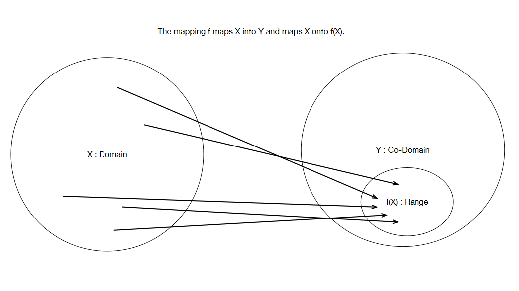
\(A\) is called the domain of \(f\) and \(B\) is called the co-domain

Example

Consider the sets \(A=\{a,b,c,d\}\) and \(B=\{1,2,3,4\}\). The following diagrams illustrate possible associations between elements of \(A\) and \(B\), i.e. domain \(A\) and co-domain \(B\):

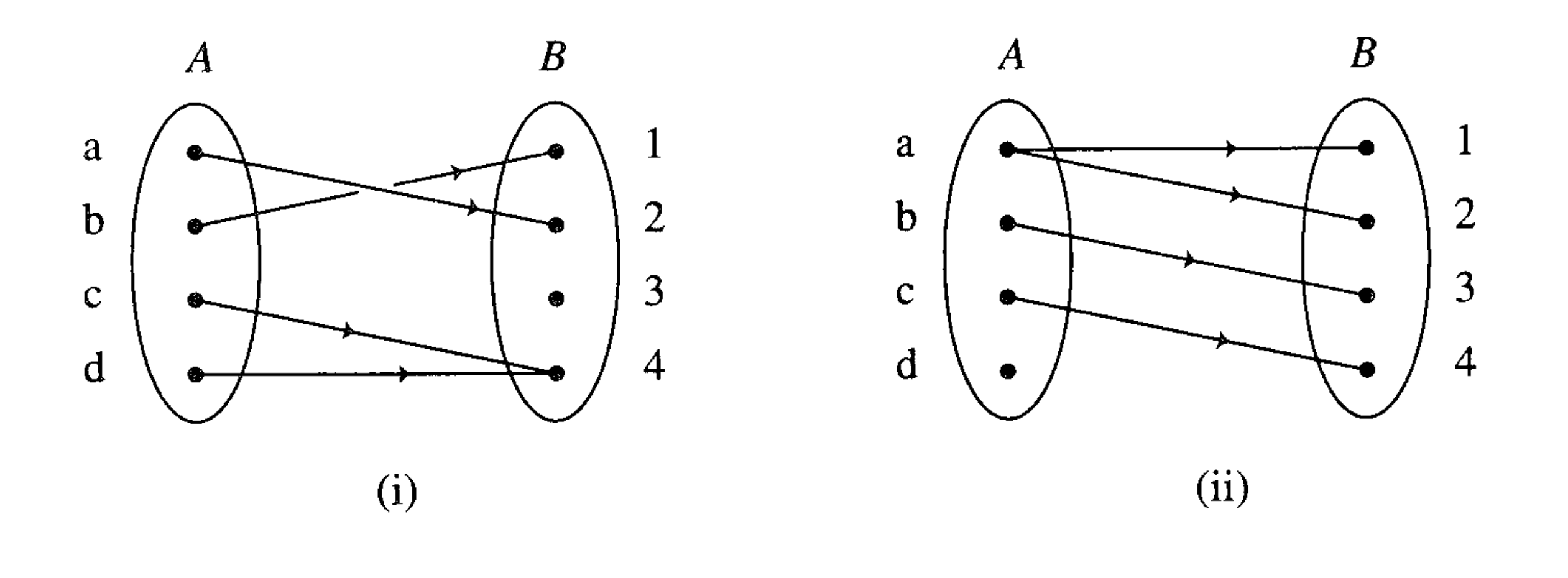
These associations can be written as subsets of the Cartesian product \(A \times B\) as follows:

• (i) \(\{(a,2),(b,1),(c,4),(d,4)\} \subset A \times B\)

• (ii) \(\{(a,1),(a,2),(b,3),(c,4)\} \subset A \times B\)

Panel (i) illustrates a function from \(A\) to \(B\) because each element of \(A\) is associated with no more than one element of \(B\).

Panel (ii) does not illustrate a function from \(A\) to \(B\) because the element \(a\) is associated with two elements of \(B\), and element \(d\) is not associated with any element of \(B\).

Example

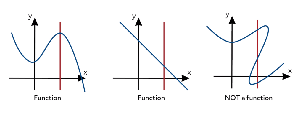
• functions have to map all elements in domain to a uniquely determined element in co-domain

Example

\[f(x) = \exp(-x^2)\]

is a function from \(\mathbb{R}\) to \(\mathbb{R}\). We may also write

\[\begin{split}f: \mathbb{R} \to \mathbb{R} \\ x \mapsto \exp(-x^2), \text{ or}\\ f: \mathbb{R} \ni x \mapsto \exp(-x^2) \in \mathbb{R} \end{split}\]

Definition

Functions can be:

• scalar-valued when \(n=1\), so \(f: A \to \mathbb{R}\)

• vector-valued when \(n>1\), so \(f: A \to \mathbb{R}^n\)

• univariate when \(A = \mathbb{R}\), so \(f: \mathbb{R} \to \mathbb{R}^n\)

• multivariate when \(A = \mathbb{R}^m\), so \(f: \mathbb{R}^m \to \mathbb{R}^n\)

Example: not a function

Definition

For each \(a \in A\), \(f(a) \in B\) is called the image of \(a\) under \(f\)

Definition

If \(f(a) = b\) then \(a\) is called a pre-image of \(b\) under \(f\)

Definition

The definitions of image and pre-image naturally generalize to subsets of the domain.

• For each \(X \subset A\), \(f(X) = \{f(x): x \in X\} \in B\) is called the image of \(X\) under \(f\)

• For each \(Y \subset B\), \(\{x: f(x) \in Y\} \in A\) is called the pre-image of \(Y\) under \(f\)

Each point in \(B\) can have one, many or zero pre-images

The co-domain of a function is not uniquely pinned down

Example

Consider the mapping defined by \(f(x) = \exp(-x^2)\)

All of these statements are valid:

• \(f\) a function from \(\mathbb{R}\) to \(\mathbb{R}\)

• \(f\) a function from \(\mathbb{R}\) to \((0, \infty)\)

• \(f\) a function from \(\mathbb{R}\) to \((0, 1]\)

Definition

The smallest possible co-domain is called the range of \(f: A \to B\):

\[ \mathrm{rng}(f) := \{ b \in B : f(a) = b \text{ for some } a \in A \} \]

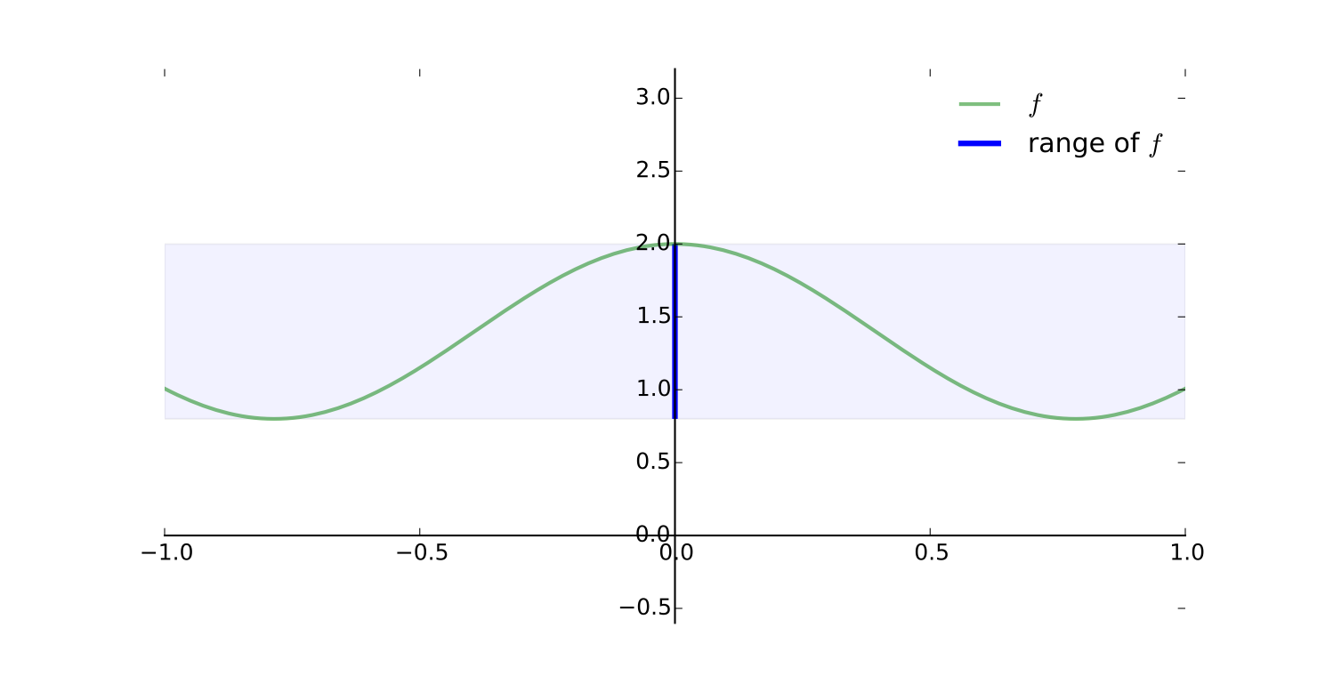
Example

Let \(f: [-1, 1] \to \mathbb{R}\) be defined by

\[ f(x) = 0.6 \cos(4 x) + 1.4 \]

Then \(\mathrm{rng}(f) = [0.8, 2.0]\)

Example

If \( f: [0, 1] \to \mathbb{R}\) is defined by

\[ f(x) = 2x \]

then \(\mathrm{rng}(f) = [0, 2]\)

Example

If \(f: \mathbb{R} \to \mathbb{R}\) is defined by

\[ f(x) = \exp(x) \]

then \(\mathrm{rng}(f) = (0, \infty)\)

Compositions

Definition

The composition of \(f: A \to B\) and \(g: B \to C\) is the function \(g \circ f\) from \(A\) to \(C\) defined by

\[ (g \circ f)(a) = g(f(a)) \quad (a \in A) \]

Example

Let \(f: \mathbb{R} \to \mathbb{R}\) be defined by \(f(x) = x^2\) and \(g: \mathbb{R} \to \mathbb{R}\) be defined by \(g(x) = x + 1\)

Then \((g \circ f)(x) = g(f(x)) = g(x^2) = x^2 + 1\)

Note that \((f \circ g)(x) = f(g(x)) = f(x+1) = (x+1)^2 \ne (g \circ f)(x)\)

• Order of components in a composite function matters

• The domain of the outer function in a composition must contain the range of the inner function

Onto (Surjections)

Definition

A function \(f: A \to B\) is called onto (or surjection) if every element of \(B\) is the image under \(f\) of at least one point in \(A\).

Equivalently, \(\mathrm{rng}(f) = B\)

Fact

\(f: A \to B\) is onto if and only if each element of \(B\) has at least one pre-image under \(f\)

Fig. 5 Onto (surjection)

Fig. 6 Not onto!

Fig. 7 Not onto!

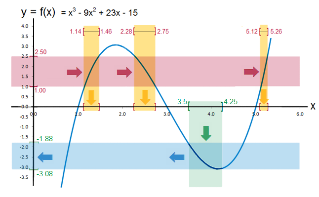
Example

The function \(f: \mathbb{R} \to \mathbb{R}\) defined by

\[ f(x) = ax^3 + b x^2 + cx + d \]

is onto whenever \(a \ne 0\)

To see this pick any \(y \in \mathbb{R}\)

We claim \(\exists \; x \in \mathbb{R}\) such that \(f(x) = y\)

Equivalent:

\[ \exists \; x \in \mathbb{R} \; \mathrm{s.t.} \; ax^3 + b x^2 + cx + d - y = 0 \]

Fact

Every cubic equation with \(a \ne 0\) has at least one real root

Fig. 8 Cubic functions from \(\mathbb{R}\) to \(\mathbb{R}\) are always onto

One-to-One (Injections)

Definition

A function \(f: A \to B\) is called one-to-one (or injection) if distinct elements of \(A\) are always mapped into distinct elements of \(B\).

That is, \(f\) is one-to-one if

\[ a \in A, \; a' \in A \text{ and } a \ne a' \implies f(a) \ne f(a') \]

Equivalently,

\[ f(a) = f(a') \implies a = a' \]

Fact

\(f: A \to B\) is one-to-one if and only if each element of \(B\) has at most one pre-image under \(f\)

Fig. 9 One-to-one

Fig. 10 One-to-one

Fig. 11 Not one-to-one

Bijections

Definition

A function that is

1. one-to-one (injection) and

2. onto (surjection)

is called a bijection or one-to-one correspondence

Fact

\(f: A \to B\) is a bijection if and only if each \(b \in B\) has one and only one pre-image in \(A\)

Example

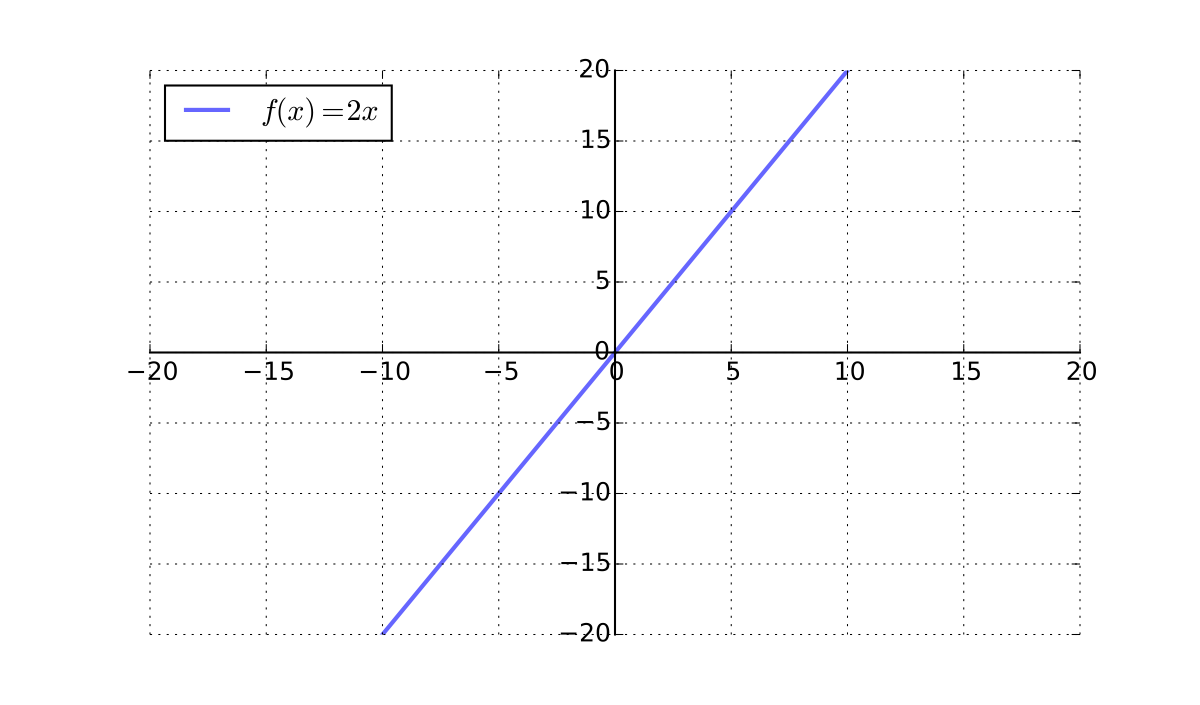
\(x \mapsto 2x\) is a bijection from \(\mathbb{R}\) to \(\mathbb{R}\)

Example

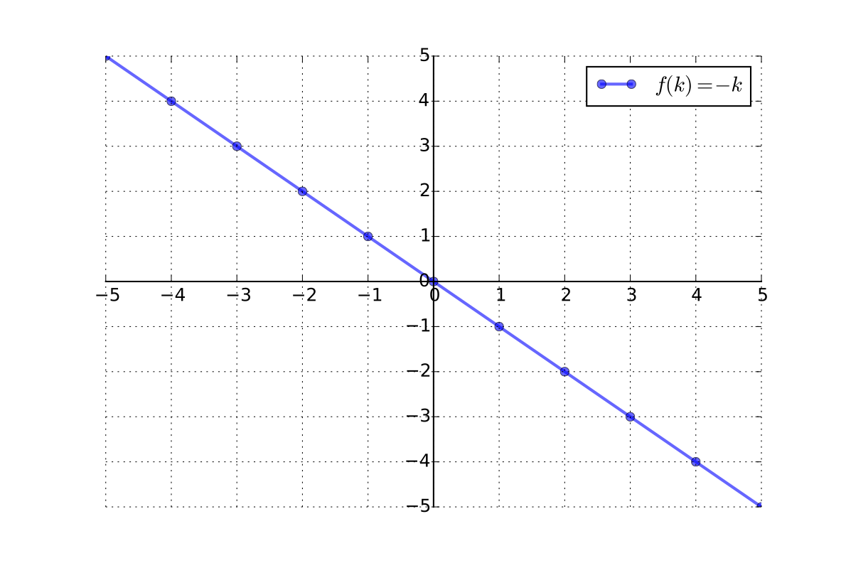
\(k \mapsto -k\) is a bijection from \(\mathbb{Z}\) to \(\mathbb{Z}\)

Example

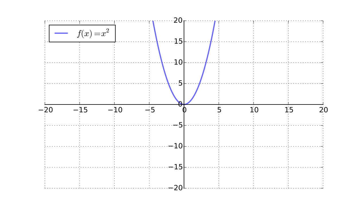
\(x \mapsto x^2\) is not a bijection from \(\mathbb{R}\) to \(\mathbb{R} \)

Inverse functions

Fact

If \(f: A \to B\) a bijection, then there exists a unique function \(\phi: B \to A\) such that

\[ \phi(f(a)) = a, \quad \forall \; a \in A \]

That function \(\phi\) is called the inverse of \(f\) and written \(f^{-1}\)

Example

Let

• \(f: \mathbb{R} \to (0, \infty)\) be defined by \(f(x) = \exp(x) := e^x\)

• \(\phi: (0, \infty) \to \mathbb{R}\) be defined by \(\phi(x) = \log(x)\)

Then \(\phi = f^{-1}\) because, for any \(a \in \mathbb{R}\),

\[ \phi(f(a)) = \log(\exp(a)) = a \]

Fact

If \(f: A \to B\) is one-to-one, then \(f: A \to \mathrm{rng}(f)\) is a bijection

Fact

Let \(f: A \to B\) and \(g: B \to C\) be bijections

1. \(f^{-1}\) is a bijection and its inverse is \(f\)

• \(f^{-1}(f(a)) = a\) for all \(a \in A\)

• \(f(f^{-1}(b)) = b\) for all \(b \in B\)

• \(g \circ f\) is a bijection from \(A\) to \(C\) and \((g \circ f)^{-1} = f^{-1} \circ g^{-1}\)

Fig. 12 Illustration of \((g \circ f)^{-1} = f^{-1} \circ g^{-1}\)

Set operations on image and pre-image

Fact

The pre-image of the union of two sets is equal to the union of the pre-images of each of the two sets: \(f^{−1}(A \cup B) = f^{−1}(A) \cup f^{−1}(B)\).

Proof

Let \(f: X \rightarrow Y\) and consider two sets, \(A \subseteq Y\) and \(B \subseteq Y\). We want to show that the pre-image of the union of two sets is equal to the union of the pre-images of each of the two sets: \(f^{−1}(A \cup B) = f^{−1}(A) \cup f^{−1}(B)\).

Note that

\[\begin{split} \begin{align*} f^{−1}(A \cup B) &= \{x \in X: f(x) \in A \cup B\} \\ &= \{x \in X : f(x) \in A \text{, or } f(x) \in B \text{, or both}\} \\ &= \{x \in X : f(x) \in A\} \cup \{x \in X : f(x) \in B\} \\ &= f^{−1}(A) \cup f^{−1}(B) \end{align*} \end{split}\]

Example

Example: \(f: \mathbb{Z} \rightarrow \mathbb{R}\) defined by \(f(z) = z^2, A = [0, 9] \subset \mathbb{R}\), and \(B = [5, 25] \subset \mathbb{R}\). \(A \cup B = [0, 25] \subset \mathbb{R}\).

The pre-image mapping here is given by \(f^{−1}(y) = \pm \sqrt{y}\) if \(\pm \sqrt{y}\) is an integer, and \(f^{−1}(y) = \varnothing\) otherwise. Note that this pre-image mapping is not an inverse function, because \(\pm \sqrt{y}\) is sometimes multi-valued.

• \(f^{−1}(A \cup B) = \{−5, −4, −3, −2, −1, 0, 1, 2, 3, 4, 5\}\)

• \(f^{−1}(A) = \{−3, −2, −1, 0, 1, 2, 3\}\)

• \(f^{−1}(B) = \{−5, −4, −3, 3, 4, 5\}\)

• \(f^{−1}(A) \cup f^{-1}(B) = \{−5, −4, −3, −2, −1, 0, 1, 2, 3, 4, 5\} = f^{−1}(A \cup B)\)

Fact

The pre-image of the intersection of two sets is equal to the intersection of the pre-images of each of the two sets: \(f^{−1}(A \cap B) = f^{−1}(A) \cap f^{−1}(B)\).

Proof

Let \(f: X \rightarrow Y\) and consider two sets, \(A \subseteq Y\) and \(B \subseteq Y\). We want to show that the pre-image of the intersection of two sets is equal to the intersection of the pre-images of each of the two sets: \(f^{−1}(A \cap B) = f^{−1}(A) \cap f^{−1}(B)\).

Note that

\[\begin{split} \begin{align*} f^{−1}(A \cap B) &= \{x \in X: f(x) \in A \cap B\} \\ &= \{x \in X : f(x) \in A \text{ and } f(x) \in B\} \\ &= \{x \in X : f(x) \in A\} \cap \{x \in X : f(x) \in B\} \\ &= f^{−1}(A) \cap f^{−1}(B) \end{align*} \end{split}\]

Example

Example: \(f: \mathbb{Z} \rightarrow \mathbb{R}\) defined by \(f(z) = z^2, A = [0, 9] \subset \mathbb{R}\), and \(B = [5, 25] \subset \mathbb{R}\). \(A \cap B = [5, 9] \subset \mathbb{R}\).

The pre-image mapping here is given by \(f^{−1}(y) = \pm \sqrt{y}\) if \(\pm \sqrt{y}\) is an integer, and \(f^{−1}(y) = \varnothing\) otherwise. Note that this pre-image mapping is not an inverse function, because \(\pm \sqrt{y}\) is sometimes multi-valued.

• \(f^{−1}(A \cap B) = \{−3, 3\}\)

• \(f^{−1}(A) = \{−3, −2, −1, 0, 1, 2, 3\}\)

• \(f^{−1}(B) = \{−5, −4, −3, 3, 4, 5\}\)

• \(f^{−1}(A) \cap f^{-1}(B) = \{−3, 3\} = f^{−1}(A \cap B)\)

Fact

The image of the union of two sets is equal to the union of the images of each of the two sets: \(f(A \cup B) = f(A) \cup f(B)\).

Proof

Let \(f: X \rightarrow Y\) and consider two sets, \(A \subseteq Y\) and \(B \subseteq Y\). We want to show that the image of the union of two sets is equal to the union of the images of each of the two sets: \(f(A \cup B) = f(A) \cup f(B)\).

Note that

\[\begin{split} \begin{align*} f(A \cup B) &= \{y \in Y: y = f(x) \text{ and } x \in A \cup B\} \\ &= \{f(x) \in Y : x \in A \cup B\} \\ &= \{f(x) \in Y : x \in A \text{, or } x \in B \text{, or both}\} \\ &= \{f(x) \in Y : x \in A\} \cup \{f(x) \in Y : x \in B\} \\ &= f(A) \cup f(B) \end{align*} \end{split}\]

Example

Example: \(f: \mathbb{Z} \rightarrow \mathbb{R}\) defined by \(f(z) = z^2, A = \{1, 2, 3\} \subset \mathbb{Z}\), and \(B = \{2,3,4,5\} \subset \mathbb{Z}\).

• \(A \cup B = \{1,2,3,4,5\} \subset \mathbb{Z}\)

• \(f(A \cup B) = \{1, 4, 9, 16, 25\} \subset \mathbb{R}\)

• \(f(A) = \{1, 4, 9\} \subset \mathbb{R}\)

• \(f(B) = \{4, 9, 16, 25\} \subset \mathbb{R}\)

• \(f(A) \cup f(B) = \{1, 4, 9, 16, 25\} = f(A \cup B)\)

Note

However, the image of the intersection of two sets is not necessarily equal to the intersection of the images of each of the two sets. In other words, there are some cases where \(f(A \cap B) \ne f(A) \cap f(B)\).

Example

Consider the mapping \(f: \mathbb{R}^2 \rightarrow \mathbb{R}\) defined by \(f(x, y) = x\), along with the sets

\[ A = \{(x, y) \in \mathbb{R}^2: x = 5, y = 5\} = \{(5, 5)\} \subset \mathbb{R}^2\]

and

\[ B = \{(x, y) \in \mathbb{R}^2: x = 5, y = 5\} = \{(5, 10)\} \subset \mathbb{R}^2\]

Note that \(A \cap B = \varnothing\), so that \(f(A \cap B) = f(\varnothing) = \varnothing\). Note also that

\[f(A) = \{f(5, 5)\} = \{5\} \subset \mathbb{R}\]

and

\[f(B) = \{f(5, 10)\} = \{5\} \subset \mathbb{R}\]

so that

\[f(A) \cap f(B) = \{5\}\]

Clearly, we have

\[f(A \cap B) = \varnothing \ne \{5\} = f(A) \cap f(B)\]

Non-decreasing and strictly increasing functions

Definition

A function \(f : X \rightarrow \mathbb{R}\), where \(X \subseteq \mathbb{R}\), is said to be a non-decreasing function if

\[x \leqslant y \iff f(x) \leqslant f(y)\]

Definition

A function \(f : X \rightarrow \mathbb{R}\), where \(X \subseteq \mathbb{R}\), is said to be a strictly increasing function if both

• (a) \(x = y \iff f(x) = f(y)\); and

• (b) \(x < y \iff f(x) < f(y)\).

Note the following:

• A strictly increasing function is also a one-to-one function.

• There are some one-to-one functions that are not strictly increasing.

• A strictly increasing function is also a non-decreasing function.

• There are some non-decreasing functions that are not strictly increasing.

Exercise: give examples of each case

Definition

Non-increasing and strictly decreasing functions are defined in a similar manner, with the inequality signs flipped.

Monotonic transformations

Suppose that \(U : X \rightarrow \mathbb{R}\) is a utility function that represents the weak preference relation \(\succsim\). This means that \(x \succsim y \iff U(x) \geqslant U(y)\).

Let \(f: \mathbb{R} \rightarrow \mathbb{R}\) be a strictly increasing function. Consider the composite function \(V = f \circ U\). It can be shown that \(V\) is also a utility function that represents the weak preference relation \(\succsim\). In other words, it can be shown that \(x \succsim y \iff V(x) \geqslant V(y)\).

Definition

Monotonic transformation of a given function is its composition with a a strictly increasing or strictly decreasing function.

Fact

Monotonic transformation of a utility function that represents a preference relation will represent the same preference relation.

Example

Consider a consumer whose preferences over bundles of strictly positive amounts of each of two commodities can be represented by a utility function \(U : \mathbb{R}^2_{++} \rightarrow \mathbb{R}_{++}\) of the form

\[U(x_1, x_2) = Ax_1^\alpha x_2^\beta\]

where \(A > 0, \alpha > 0\), and \(\beta > 0\).

Such preferences are known as Cobb-Douglas preferences.

• The function \(f: \mathbb{R}_{++} \rightarrow \mathbb{R}_{++}\) defined by \(f(x) = \left( \frac{1}{A} \right)x\) is strictly increasing. Thus we know that another utility function that represents this consumer’s preferences is

\[V(x_1, x_2) = f(U((x_1, x_2)) = \left( \frac{1}{A} \right) (Ax_1^\alpha x_2^\beta) = x_1^\alpha x_2^\beta\]

• The function \(g: \mathbb{R}_{++} \rightarrow \mathbb{R}_{++}\) defined by \(g(x) = x^{\frac{1}{(\alpha + \beta)}}\) is strictly increasing. (If any relevant surd expression can be either positive or negative, then we will assume that the positive option is chosen throughout this Cobb-Douglas preferences example.) Thus we know that another utility function that represents this consumer’s preferences is

\[W(x_1, x_2) = g(V((x_1, x_2)) = (x_1^\alpha x_2^\beta)^{\frac{1}{(\alpha + \beta)}} = x_1^\gamma x_2^{(1 - \gamma)}\]

where \( \gamma = \frac{\alpha}{\alpha + \beta} \in (0, 1)\).

• The function \(k: \mathbb{R}_{++} \rightarrow \mathbb{R}\) defined by \(k(x) = ln(x )\) is strictly increasing. Thus we know that another utility function that represents this consumer’s preferences is

\[Z(x_1, x_2) = k(W((x_1, x_2)) = ln (x_1^\gamma x_2^{(1 - \gamma)})\]

\[= \gamma \; ln(x_1) + (1 − \gamma) \; ln(x_2) \]

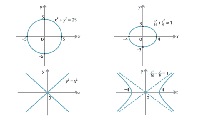
Graphs of functions and correspondences

Definition

A graph of a mapping \(f \colon X \to Y\) is a set \(\Gamma \subset X \times Y\) of points \(x \in X\) and \(y \in Y\) where it holds \(y \in f(x)\), or \(y = f(x)\) in hte case \(f\) is a function.

For the functions \(\mathbb{R} \to \mathbb{R}\) a graph can be conveniently drawn on a plane. We can also easily plot graphs of correspondences \(\mathbb{R} \to 2^\mathbb{R}\).

Example

Fig. 13 Graphs of various functions

Fig. 14 Graphs of various correspondences

Shifting the graph

Fact

Consider \(\Gamma_0\) the graph of function \(f(x): \mathbb{R} \to \mathbb{R}\). Denote \(\Gamma_1\) the graph of the composite function \(g(x) = af(bx+c)+d\), such that when \(a=b=1\) and \(c=d=0\) \(f(x)=g(x)\). It holds that:

• for \(a \ne 1\), \(a>0\) graph \(\Gamma_1\) is a vertical stretch or compression of \(\Gamma_0\) by a factor of \(|a|\)

• for \(a<0\) in addition graph \(\Gamma_1\) flips around the horizontal axis

• for \(b \ne 1\), \(b>0\) graph \(\Gamma_1\) is a horizontal stretch or compression of \(\Gamma_0\) by a factor of \(|b|\)

• for \(b<0\) in addition graph \(\Gamma_1\) flips around the vertical axis

• for \(c \ne 0\) graph \(\Gamma_1\) is a horizontal shift of \(\Gamma_0\) by \(\frac{c}{b}\), left for \(\frac{c}{b}>0\) and right for \(\frac{c}{b}<0\)

• for \(d \ne 0\) graph \(\Gamma_1\) is a vertical shift of \(\Gamma_0\) by \(d\), up for \(d>0\) and down for \(d<0\)

Example

Online graphing tools like Desmos

Graph of the inverse function

Fact

When the inverse exists, its graph is a flip of the original graph over the 45 degree line.

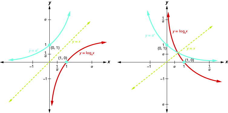
Fig. 15 Graph of inverse functions