📖 Univariate differentiation

⏱ | words

References and additional materials

[Sydsæter, Hammond, Strøm, and Carvajal, 2016]

Chapters 6.1-6.4, 6.6-6.9, 7.4-7.6

• Great video on Taylor series YouTube Morphocular

Definition

Consider a function \(f : X \rightarrow \mathbb{R}\), where \(X \subseteq \mathbb{R}\). Let \((x_0, f (x_0))\) and \((x_0 + h, f (x_0 + h))\) be two points that lie on the graph of this function.

Draw a straight line between these two points. The slope of this line is

\[\begin{split} \begin{align*} \frac{\text{rise}}{\text{run}} &= \frac{y_2 − y_1}{x_2 − x_1} \\ &= \frac{f (x_0 + h) − f (x_0)}{x_0 + h − x_0} \\ &= \frac{f (x_0 + h) − f (x_0)}{h} \end{align*} \end{split}\]

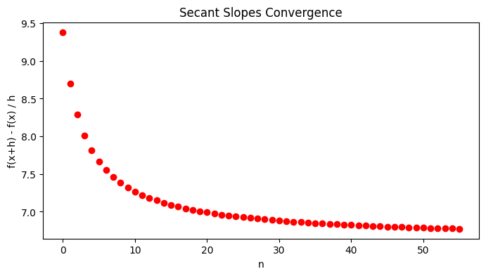
What happens to this slope as \(h \rightarrow 0\) (that is, as the second point gets very close to the first point?

Let \(h = 1/n\) and look at the limit as \(n \to \infty\)

Show code cell source Hide code cell source

import numpy as np
import matplotlib.pyplot as plt

# Define the function and its derivative
def f(x):
    return np.exp(np.exp(x))  # Example function

# Point of tangency
a = 0.4 
fa = f(a)

# Values for secant points approaching 'a'
h_values = 1/np.arange(4, 60)

secant_slopes = np.empty(len(h_values))

for i,h in enumerate(h_values):
    x1, x2 = a, a + h
    y1, y2 = f(x1), f(x2)
    secant_slopes[i] = (y2 - y1) / (x2 - x1)

# Plot convergence of secant to tangent
plt.figure(figsize=(8, 4))
plt.scatter(np.arange(len(h_values)), secant_slopes, color='red')

# Labels and legend
plt.xlabel('n')
plt.ylabel('f(x+h) - f(x) / h')
plt.title('Secant Slopes Convergence')
# plt.grid(True)
plt.show()

Show code cell source Hide code cell source

import numpy as np
import matplotlib.pyplot as plt

def f(x):
  return np.exp(x)  # Example function

def df(x):
  return np.exp(x)  # Derivative (tangent slope)

# Point of tangency
a = 0.4 
fa = f(a)

# Generate x values for the plot
x_vals = np.linspace(0, 3, 400)
y_vals = f(x_vals)

# Values for secant points approaching 'a'
h_values = [2.5,2,1.5,1,0.5]

plt.figure(figsize=(8, 6))

# Plot the function
plt.plot(x_vals, y_vals, label=r'$f(x) = exp(x)$', color='black', linewidth=2)


# Plot secant lines for different h values
for h in h_values:
  x1, x2 = a, a + h
  y1, y2 = f(x1), f(x2)
  
  # Slope of secant line
  secant_slope = (y2 - y1) / (x2 - x1)
  
  # Equation of secant line
  secant_x = np.linspace(0, x2+0.2, 100)
  secant_y = fa + secant_slope * (secant_x - a)
  
  plt.plot(secant_x, secant_y, linestyle='--', label=f'Secant h={h:.2f}')


# Plot the tangent line
tangent_slope = df(a)
tangent_x = np.linspace(0, a + 2.5, 100)
tangent_y = fa + tangent_slope * (tangent_x - a)
plt.plot(tangent_x, tangent_y, 'r', label='Tangent at x=1', linewidth=1.5)


# Highlight the point of tangency
plt.scatter([a], [fa], color='red', zorder=5, label='Point of Tangency')

# Labels and legend
plt.xlabel('x')
plt.ylabel('f(x)')
plt.title('Secant Converging to Tangent')
plt.legend()
plt.grid(True)
plt.show()

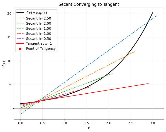
Definition

The (first) derivative of the function \(f(x)\) at the point \(x=x_{0}\), if it exists, is defined to be

\[ f^{\prime}\left(x_{0}\right) =\frac{d f}{d x}(x_{0}) =\lim _{h \rightarrow 0} \frac{f\left(x_{0}+h\right)-f\left(x_{0}\right)}{h} . \]

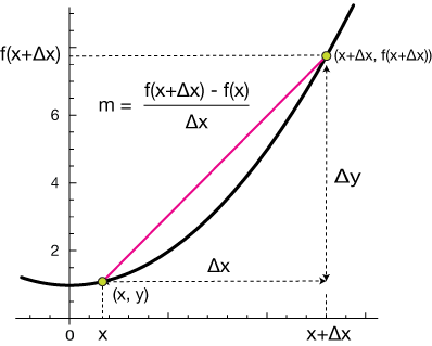
This is simply the slope of the straight line that is tangent to the function \(f(x)\) at the point \(x=x_{0}\).

Differentiation from first principles

We will now proceed to use this definition to find the derivative of some simple functions. This is sometimes called “finding the derivative of a function from first principles”.

Example: the derivative of a constant function

Consider the function \(f: X \longrightarrow \mathbb{R}\) defined by \(f(x)=b\), where \(b \in \mathbb{R}\) is a constant. Clearly we have \(f\left(x_{0}\right)=f\left(x_{0}+h\right)=b\) for all choices of \(x_{0}\) and \(h\).

Thus we have

\[ \frac{f\left(x_{0}+h\right)-f\left(x_{0}\right)}{h}=\frac{b-b}{h}=\frac{0}{h}=0 \]

for all choices of \(x_{0}\) and \(h\).

This means that

\[ \lim _{h \rightarrow 0} \frac{f\left(x_{0}+h\right)-f\left(x_{0}\right)}{h}=\lim _{h \rightarrow 0} 0=0 \]

As such, we can conclude that

\[ f^{\prime}(x)=\frac{d f}{d x}=0 \]

Example: the derivative of a linear function

Consider the function \(f: X \longrightarrow \mathbb{R}\) defined by \(f(x)=a x+b\). Note that

\[\begin{split} \begin{aligned} f(x+h) & =a(x+h)+b \\ & =a x+a h+b \\ & =a x+b+a h \\ & =f(x)+a h . \end{aligned} \end{split}\]

Thus we have

\[ \frac{f(x+h)-f(x)}{h}=\frac{f(x)+a h-f(x)}{h}=\frac{a h}{h}=a . \]

This means that \(\lim _{h \rightarrow 0} \frac{f\left(x_{0}+h\right)-f\left(x_{0}\right)}{h}=\lim _{h \rightarrow 0} a=a\).

As such, we can conclude that \(f^{\prime}(x)=\frac{d f}{d x}=a\).

Example: the derivative of a quadratic power function

Consider the function \(f: X \longrightarrow \mathbb{R}\) defined by \(f(x)=x^{2}\). Note that

\[\begin{split} \begin{aligned} f(x+h) & =(x+h)^{2} \\ & =x^{2}+2 x h+h^{2} \\ & =f(x)+2 x h+h^{2} \end{aligned} \end{split}\]

Thus we have

\[\begin{split} \begin{aligned} \frac{f(x+h)-f(x)}{h} & =\frac{f(x)+2 x h+h^{2}-f(x)}{h} \\ & =\frac{2 x h+h^{2}}{h} \\ & =2 x+h . \end{aligned} \end{split}\]

This means that \(\lim _{h \rightarrow 0} \frac{f\left(x_{0}+h\right)-f\left(x_{0}\right)}{h}=\lim _{h \rightarrow 0}(2 x+h)=2 x\).

As such, we can conclude that \(f^{\prime}(x)=\frac{d f}{d x}=2 x\)

Example: the derivative of a quadratic polynomial function

Consider the function \(f: X \longrightarrow \mathbb{R}\) defined by \(f(x)=a x^{2}+b x+c\). Note that

\[\begin{split} \begin{aligned} f(x+h) & =a(x+h)^{2}+b(x+h)+c \\ & =a\left(x^{2}+2 x h+h^{2}\right)+b x+b h+c \\ & =a x^{2}+2 a x h+a h^{2}+b x+b h+c \\ & =\left(a x^{2}+b x+c\right)+(2 a x+b) h+a h^{2} \\ & =f(x)+(2 a x+b) h+a h^{2} . \end{aligned} \end{split}\]

Thus we have

\[\begin{split} \begin{aligned} \frac{f(x+h)-f(x)}{h} & =\frac{f(x)+(2 a x+b) h+a h^{2}-f(x)}{h} \\ & =\frac{(2 a x+b) h+a h^{2}}{h} \\ & =(2 a x+b)+a h \\ & =2 a x+b+a h . \end{aligned} \end{split}\]

This means that

\[ \lim _{h \rightarrow 0} \frac{f\left(x_{0}+h\right)-f\left(x_{0}\right)}{h}=\lim _{h \rightarrow 0}(2 a x+b+a h)=2 a x+b \]

As such, we can conclude that \(f^{\prime}(x)=\frac{d f}{d x}=2 a x+b\).

Fact (Binomial theorem)

Suppose that \(x, y \in \mathbb{R}\) and \(n \in \mathbb{Z}_+ = \mathbb{N} \cup \{0\}\).

We have

\[ (x + y)^n = \sum_{k = 0}^{n} \binom{n}{k} x^{(n−k)} y^k \]

where \(\binom{n}{k} = C_{n,k} = \frac{n!}{k! (n − k)!}\) is known as a binomial coefficient (read “\(n\) choose \(k\)” because this is the number of ways to choose a subset of \(k\) elements from a set of \(n\) elements). \(n! = \prod_{k=1}^n k\) denotes a factorial of \(n\), and \(0! = 1\) by definition.

Useful property is \(\binom{n}{k} = C_{n,k} = C_{n-1,k-1}+C_{n-1,k}\) is illustrated by Pascal’s triangle.

Example: the derivative of a positive integer power function

Consider the function \(f: \mathbb{R} \longrightarrow \mathbb{R}\) defined by \(f(x)=x^{n}\), where \(n \in \mathbb{N}=\mathbb{Z}_{++}\). We know from the binomial theorem that

\[\begin{split} \begin{aligned} f(x+h) & =(x+h)^{n} \\ & =\sum_{r=0}^{n}\left(\begin{array}{l} n \\ r \end{array}\right) x^{n-r} h^{r} \\ & =\left(\begin{array}{l} n \\ 0 \end{array}\right) x^{n} h^{0}+\sum_{r=1}^{n}\left(\begin{array}{l} n \\ r \end{array}\right) x^{n-r} h^{r} \\ & =1 x^{n}(1)+\sum_{r=1}^{n}\left(\begin{array}{l} n \\ r \end{array}\right) x^{n-r} h^{r} \\ & =x^{n}+\sum_{r=1}^{n}\left(\begin{array}{l} n \\ r \end{array}\right) x^{n-r} h^{r} . \end{aligned} \end{split}\]

Thus we have

\[\begin{split} \begin{aligned} \frac{f(x+h)-f(x)}{h} & =\frac{f(x)+\sum_{r=1}^{n}\left(\begin{array}{l} n \\ r \end{array}\right) x^{n-r} h^{r}-f(x)}{h} \\ & =\frac{\sum_{r=1}^{n}\left(\begin{array}{l} n \\ r \end{array}\right) x^{n-r} h^{r}}{h} \\ & =\sum_{r=1}^{n}\left(\begin{array}{l} n \\ r \end{array}\right) x^{n-r} h^{r-1} \\ & =\left(\begin{array}{l} n \\ 1 \end{array}\right) x^{n-1} h^{0}+\sum_{r=2}^{n}\left(\begin{array}{l} n \\ r \end{array}\right) x^{n-r} h^{r-1} \\ & =n x^{n-1}(1)+\sum_{r=2}^{n}\left(\begin{array}{l} n \\ r \end{array}\right) x^{n-r} h^{r-1} \end{aligned} \end{split}\]

\[\begin{split} \frac{f(x+h)-f(x)}{h} & =n x^{n-1}+\sum_{r=2}^{n}\left(\begin{array}{l} n \\ r \end{array}\right) x^{n-r} h^{r-1} \end{split}\]

This means that

\[\begin{split} \lim _{h \rightarrow 0} \frac{f\left(x_{0}+h\right)-f\left(x_{0}\right)}{h}=\lim _{h \rightarrow 0}\left(n x^{n-1}+\sum_{r=2}^{n}\left(\begin{array}{l} n \\ r \end{array}\right) x^{n-r} h^{r-1}\right)=n x^{n-1} \end{split}\]

As such, we can conclude that

\[ f^{\prime}(x)=\frac{d f}{d x}=n x^{n-1} \]

Example: derivative of an \(e^x\)

Consider the function \(f: \mathbb{R} \longrightarrow \mathbb{R}_{++}\) defined by \(f(x)=e^x\), where \(e\) in Euler’s constant. Recall that by definition \(e = \lim_{n \to \infty} (1+\frac{1}{n})^n\)

\[ \lim_{h \to 0} \frac{f(x+h)-f(x)}{h} =\lim_{h \to 0} \frac{e^{x+h}-e^x}{h} =\lim_{h \to 0} \frac{e^x(e^h-1)}{h} \]

Consider \(\lim_{h \to 0}\frac{e^h-1}{h}\) after substitution \(t=(e^h-1)^{-1}\) \(\Leftrightarrow\) \(h = \ln(t^{-1}+1)\)

\[\begin{split} \begin{array}{l} \lim_{h \to 0}\frac{e^h-1}{h} = \lim_{t \to \infty}\frac{t^{-1}}{\ln(t^{-1}+1)} =\\= \lim_{t \to \infty}\left(t \ln(t^{-1}+1) \right)^{-1} =\\= \Big( \ln \Big[ \lim_{t \to \infty} (1+\frac{1}{t})^t \Big] \Big)^{-1} =\\= ( \ln e )^{-1}= (1)^{-1} = 1 \end{array} \end{split}\]

We used the fact that of \(e = \lim_{n \to \infty} (1+1/n)^n\).

Therefore

\[ \lim_{h \to 0} \frac{f(x+h)-f(x)}{h} =\lim_{h \to 0} \frac{e^x(e^h-1)}{h} = e^x \lim_{h \to 0} \frac{e^h-1}{h} = e^x \]

Differentiation rules

Fact: The derivatives of some commonly encountered functions

• If \(f(x)=a\), where \(a \in \mathbb{R}\) is a constant, then \(f^{\prime}(x)=0\).

• If \(f(x)=a x+b\), then \(f^{\prime}(x)=a\).

• If \(f(x)=a x^{2}+b x+c\), then \(f^{\prime}(x)=2 a x+b\).

• If \(f(x)=x^{n}\), where \(n \in \mathbb{N}\), then \(f^{\prime}(x)=n x^{n-1}\).

• If \(f(x)=\frac{1}{x^{n}}=x^{-n}\), where \(n \in \mathbb{N}\), then \(f^{\prime}(x)=-n x^{-n-1}=-n x^{-(n+1)}=\frac{-n}{x^{n+1}}\). (Note that we need to assume that \(x \neq 0\).)

• If \(f(x)=e^{x}=\exp (x)\), then \(f^{\prime}(x)=e^{x}=\exp (x)\).

• If \(f(x)=\ln (x)\), then \(f^{\prime}(x)=\frac{1}{x}\). (Recall that \(\ln (x)\) is only defined for \(x>0\), so we need to assume that \(x>0\) here.)

Fact: Scalar Multiplication Rule

If \(f(x)=c g(x)\) where \(c \in \mathbb{R}\) is a constant, then

\[ f^{\prime}(x)=c g^{\prime}(x) \]

Example

Let \(f(x) = a g(x)\) where \(g(x)=x\). From the derivation of the derivative of the linear functions we know that \(g'(x) = 1\) and \(f'(x) = a\). We can verify that \(f'(x) = a g'(x)\).

Fact: Summation Rule

If \(f(x)=g(x)+h(x)\), then

\[ f^{\prime}(x)=g^{\prime}(x)+h^{\prime}(x) \]

Example

Let \(f(x) = a x + b\) and \(g(x)=cx+d\). From the derivation of the derivative of the linear functions we know that \(f'(x) = a\) and \(g'(x) = c\). The sum \(f(x)+g(x) = (a+c)x+b+d\) is also a linear function, therefore \(\frac{d}{dx}\big(f(x)+g(x)\big) = a+c\).

We can thus verify that \(\frac{d}{dx}\big(f(x)+g(x)\big) = f'(x)+ g'(x)\).

Fact: Product Rule

If \(f(x)=g(x) h(x)\), then

\[ f^{\prime}(x)=g^{\prime}(x) h(x)+h^{\prime}(x) g(x) \]

Example

Let \(f(x) = x\) and \(g(x)=x\). From the derivation of the derivative of the linear functions we know that \(f'(x) = g'(x) = 1\). The product \(f(x)g(x) = x^2\) and from the derivation of above we know that \(\frac{d}{dx}\big(f(x)g(x)\big) = \frac{d}{dx}\big(x^2\big) = 2x\).

Using the product formula we can verify \(\frac{d}{dx}\big(f(x)g(x)\big) = 1\cdot x + x \cdot 1 = 2x\).

Fact: Quotient Rule

If \(f(x)=\frac{g(x)}{h(x)}\), then

\[ f^{\prime}(x)=\frac{g^{\prime}(x) h(x)-h^{\prime}(x) g(x)}{[h(x)]^{2}} \]

The quotient rule is redundant

In a sense, the quotient rule is redundant. The reason for this is that it can be obtained from a combination of the product rule and the chain rule.

Suppose that \(f(x)=\frac{g(x)}{h(x)}\). Note that

\[ f(x)=\frac{g(x)}{h(x)}=g(x)[h(x)]^{-1} \]

Let \([h(x)]^{-1}=k(x)\). We know from the chain rule that

\[ k^{\prime}(x)=(-1)[h(x)]^{-2} h^{\prime}(x)=\frac{-h^{\prime}(x)}{[h(x)]^{2}} \]

Note that

\[ f(x)=\frac{g(x)}{h(x)}=g(x)[h(x)]^{-1}=g(x) k(x) \]

We know from the product rule that

\[\begin{split} \begin{aligned} f^{\prime}(x) & =g^{\prime}(x) k(x)+k^{\prime}(x) g(x) \\ & =g^{\prime}(x)[h(x)]^{-1}+\left(\frac{-h^{\prime}(x)}{[h(x)]^{2}}\right) g(x) \\ & =\frac{g^{\prime}(x)}{h(x)}-\frac{h^{\prime}(x) g(x)}{[h(x)]^{2}} \\ & =\frac{g^{\prime}(x) h(x)}{[h(x)]^{2}}-\frac{h^{\prime}(x) g(x)}{[h(x)]^{2}} \\ & =\frac{g^{\prime}(x) h(x)-h^{\prime}(x) g(x)}{[h(x)]^{2}} . \end{aligned} \end{split}\]

This is simply the quotient rule!

Fact: Chain Rule

If \(f(x)=g(h(x))\), then

\[ f^{\prime}(x)=g^{\prime}(h(x)) h^{\prime}(x) \]

Example: the derivative of an exponential function

Suppose that \(f(x)=a^{x}\), where \(a \in \mathbb{R}_{++}=(0, \infty)\) and \(x \neq 0\).

We can write \(f(x) = e^{\ln a^{x}} = e^ {x \ln(a)}\), and using the chain rule

\[ f'(x) = \frac{d}{dx} e^ {x \ln(a)} = e^ {x \ln(a)} \frac{d}{dx} (x \ln(a)) = a^x \ln(a) \]

Fact: The Inverse Function Rule

Suppose that the function \(y=f(x)\) has a well defined inverse function \(x=f^{-1}(y)\). If appropriate regularity conditions hold, then

\[ \frac{dx}{d y} = \frac{d}{d y} f^{-1}(y) =\frac{1}{f'\big( f^{-1}(y)\big)} \]

Example: the derivative of a logarithmic function

Suppose that \(f(x)=\log _{a}(x)\), where \(a \in \mathbb{R}_{++}=(0, \infty)\) and \(x>0\).

Recall that \(y = \log _{a}(x) \iff a^y = x\). Then evaluating \(\frac{dx}{dy}\) using the derivative of the exponential function we have

\[ \frac{dx}{dy} = a^y \ln(a) \]

On the other hand, using the inverse function rule we have

\[ \frac{dx}{dy} = \frac{1}{f'(a^y)} \]

Combining the two expressions and reinserting \(a^y = x\), we have

\[ f'(x) = \frac{d \log_a(x)}{d x} = \frac{1}{a^y \ln(a)} = \frac{1}{x \ln(a)} \]

Example: product rule

Consider the function \(f(x)=(a x+b)(c x+d)\).

Differentiation Approach One: Note that

\[\begin{split} \begin{aligned} f(x) & =(a x+b)(c x+d) \\ & =a c x^{2}+a d x+b c x+b d \\ & =a c x^{2}+(a d+b c) x+b d \end{aligned} \end{split}\]

Thus we have

\[\begin{split} \begin{aligned} f^{\prime}(x) & =2 a c x+(a d+b c) \\ & =2 a c x+a d+b c \end{aligned} \end{split}\]

Differentiation Approach Two: Note that \(f(x)=g(x) h(x)\) where \(g(x)=a x+b\) and \(h(x)=c x+d\). This means that \(g^{\prime}(x)=a\) and \(g^{\prime}(x)=c\). Thus we know, from the product rule, that

\[\begin{split} \begin{aligned} f^{\prime}(x) & =g^{\prime}(x) h(x)+h^{\prime}(x) g(x) \\ & =a(c x+d)+c(a x+b) \\ & =a c x+a d+a c x+b c \\ & =2 a c x+a d+b c . \end{aligned} \end{split}\]

Differentiability and continuity

• Continuity is a necessary, but not sufficient, condition for differentiability.

  • Being a necessary condition means that “not continuous” implies “not differentiable”, which means that differentiable implies continuous.

  • Not being a sufficient condition means that continuous does NOT imply differentiable.

• Differentiability is a sufficient, but not necessary, condition for continuity.

  • Being a sufficient condition means that differentiable implies continuous.

  • Not being a necessary condition means that “not differentiable” does NOT imply “not continuous”, which means that continuous does NOT imply differentiable.

Continuity does NOT imply differentiability

To support this statement all we need is to demonstrate a single example of a function that is continuous at a point but not differentiable at that point.

Proof

Consider the function

\[\begin{split} f(x)=\left\{\begin{array}{cc} 2 x & \text { if } x \leqslant 1 \\ \frac{1}{2} x+\frac{3}{2} & \text { if } x \geq 1 \end{array}\right. \end{split}\]

(There is no problem with this double definition at the point \(x=1\) because the two parts of the function are equal at that point.)

This function is continuous at \(x=1\) because

\[ \lim _{x \rightarrow 1} 2 x=2=\lim _{x \rightarrow 1}\left(\frac{1}{2} x+\frac{3}{2}\right) \]

and

\[ f(1)=2 \]

However, this function is not differentiable at \(x=1\). To show this it is convenient to use the Heine definition of the limit for a function in application to the derivative.

Consider two sequence converging to \(x=1\) from two different directions:

\[ \{p_n\}_{n \in \mathbb{N}}: p_n < 0, p_n \to 0, \quad \{q_n\}_{n \in \mathbb{N}}: q_n > 0, q_n \to 0 \]

Then at \(x=1\)

\[ \lim_{n \to \infty} \frac{f(1+p_n)-f(1)}{p_n} = \lim_{n \to \infty} \frac{2+2p_n-2}{p_n} = 2 \]

but

\[ \lim_{n \to \infty} \frac{f(1+q_n)-f(1)}{q_n} = \lim_{n \to \infty} \frac{\frac{1}{2} +\frac{1}{2}q_n+\frac{3}{2} - \frac{1}{2} - \frac{3}{2}}{q_n} = \frac{1}{2} \]

Thus, for two different convergent sequences \(p_n\) and \(q_n\) we have two different limits of the derivative at \(x=1\). We conclude that the limit \(\lim _{h \rightarrow 1} \frac{f(1+h)-f(1)}{h}\) is undefined.

\(\blacksquare\)

Example

A example of a function that is continuous at every point but not differentiable at any point is the Wiener process (Brownian motion).

Differentiability implies continuity

Proof

Consider a function \(f: X \longrightarrow \mathbb{R}\) where \(X \subseteq \mathbb{R}\). Suppose that

\[ \lim _{h \rightarrow 0}\left(\frac{f(a+h)-f(a)}{h}\right) \]

exists.

We want to show that this implies that \(f(x)\) is continuous at the point \(a \in X\). The following proof of this proposition is drawn from [Ayres Jr and Mendelson, 2013] (Chapter 8, Solved Problem 2).

First, note that

\[\begin{split} \begin{gathered} \lim _{h \rightarrow 0}(f(a+h)-f(a))=\lim _{h \rightarrow 0}\left\{\left(\frac{h}{h}\right)(f(a+h)-f(a))\right\} \\ =\lim _{h \rightarrow 0}\left\{h\left(\frac{f(a+h)-f(a)}{h}\right)\right\} \\ =\lim _{h \rightarrow 0}(h) \lim _{h \rightarrow 0}\left(\frac{f(a+h)-f(a)}{h}\right) \\ =(0)\left(\lim _{h \rightarrow 0}\left(\frac{f(a+h)-f(a)}{h}\right)\right) \\ =0 . \end{gathered} \end{split}\]

Thus we have

\[ \lim _{h \rightarrow 0}(f(a+h)-f(a))=0 . \]

Now note that

\[\begin{split} \begin{gathered} \lim _{h \rightarrow 0}(f(a+h)-f(a))=\lim _{h \rightarrow 0} f(a+h)-\lim _{h \rightarrow 0} f(a) \\ =\left(\lim _{h \rightarrow 0} f(a+h)\right)-f(a) \end{gathered} \end{split}\]

Upon combining these two results, we obtain

\[ \left(\lim _{h \rightarrow 0} f(a+h)\right)-f(a)=0 \Longleftrightarrow \lim _{h \rightarrow 0} f(a+h)=f(a) . \]

Finally, note that

\[ \lim _{x \rightarrow a} f(x)=\lim _{h \rightarrow 0} f(a+h) . \]

Thus we have

\[ \lim _{x \rightarrow a} f(x)=f(a) \]

This means that \(f(x)\) is continuous at the point \(x=a\).

\(\blacksquare\)

Higher-order derivatives

Suppose that \(f: X \longrightarrow \mathbb{R}\), where \(X \subseteq \mathbb{R}\), is an \(n\)-times continuously differentiable function for some \(n \geqslant 2\).

We can view the first derivative of this function as a function in its own right. This can be seen by letting \(g(x)=f^{\prime}(x)\).

The second derivative of \(f(x)\) with respect to \(x\) twice is simply the first derivative of \(g(x)\) with respect to \(x\).

In other words,

\[ f^{\prime \prime}(x)=g^{\prime}(x) \]

or, if you prefer,

\[ \frac{d^{2} f}{d x d x}=\frac{d g}{d x} \]

Thus we have

\[ \frac{d^{2} f}{d x d x}=\frac{d}{d x}\left(\frac{d f}{d x}\right) \]

The same approach can be used for defining third and higher order derivative.

Definition

The \(n\)-th order derivative of a function \(f \colon \mathbb{R} \to \mathbb{R}\), if it exists, is the derivative of it’s \((n-1)\)-th order derivative treated as an independent function.

\[ f^{(k)}(x)=\frac{d^{k} f}{\underbrace{dx \cdots dx}_{k}}= \frac{d}{d x}\left(\frac{d^{k-1} f}{\underbrace{dx \cdots dx}_{k-1}}\right) \]

for all \(k \in\{1,2, \cdots, n\}\), where we define

\[ f^{(0)}(x)=f(x) \]

Example

• Let \(f(x)=x^{n}\)

• Then we have:

• \(f^{\prime}(x)=\frac{d f(x)}{d x}=n x^{n-1}\)

• \(f^{\prime \prime}(x)=\frac{d f^{\prime}(x)}{d x}=n(n-1) x^{n-2}\),

• \(f^{\prime \prime \prime}(x)=\frac{d f^{\prime \prime}(x)}{d x}=n(n-1)(n-2) x^{n-3}\),

• and so on and so forth until

• \(f^{(k)}(x)=\frac{d f^{(k-1)}(x)}{d x}=n(n-1)(n-2) \cdots(n-(k-1)) x^{n-k}\),

• and so on and so forth until

• \(f^{(n)}(x)=\frac{d f^{(n-1)}(x)}{d x}=n(n-1)(n-2) \cdots(1) x^{0}\).

• Note that \(n(n-1)(n-2) \cdots(1)=n\) ! and \(x^{0}=1\) (asuming that \(x \neq 0\) ).

• This means that \(f^{(n)}(x)=n\) !, which is a constant.

• As such, we know that \(f^{(n+1)}(x)=\frac{d f^{(n)}(x)}{d x}=0\).

• This means that \(f^{(n+j)}(x)=0\) for all \(j \in \mathbb{N}\).

Taylor series

Definition

The function \(f: X \to \mathbb{R}\) is said to be of differentiability class \(C^m\) if derivatives \(f'\), \(f''\), \(\dots\), \(f^{(m)}\) exist and are continuous on \(X\)

Fact

Consider \(f: X \to \mathbb{R}\) and let \(f\) to be a \(C^m\) function. Assume also that \(f^{(m+1)}\) exists, although may not necessarily be continuous.

For any \(x,a \in X\) there is such \(z\) between \(a\) and \(x\) that

\[\begin{split}\begin{array}{rl} f(x) =& f(a) + f'(a)(x-a) + \dots + \frac{f^{(m)}(a)}{m!}(x-a)^m + R_m(x) =\\ =& f(a) + \sum_{k=1}^m \frac{f^{(k)}(a)}{k!}(x-a)^k + R_m(x), \end{array}\end{split}\]

where the remainder is given by

\[R_m(x) = \frac{f^{(m+1)}(z)(x-a)^{m+1}}{(m+1)!} = o\big((x-a)^m\big)\]

Definition

Little-o notation is used to describe functions that approach zero faster than a given function

\[f(x) = o\big(g(x)\big) \; \text{as} \; x \to a \quad \iff \quad \lim_{x \to a} \frac{f(x)}{g(x)} = 0\]

Loosely speaking, if \(f \colon \mathbb{R} \to \mathbb{R}\) is suitably differentiable at \(a\), then

\[ f(x) \approx f(a) + f'(a)(x-a) \]

for \(x\) very close to \(a\),

\[ f(x) \approx f(a) + f'(a)(x-a) + \frac{f''(a)}{2!}(x-a)^2 \]

on a slightly wider interval, etc.

These are the 1st and 2nd order Taylor series approximations to \(f\) at \(a\) respectively

As the order goes higher we get better approximation

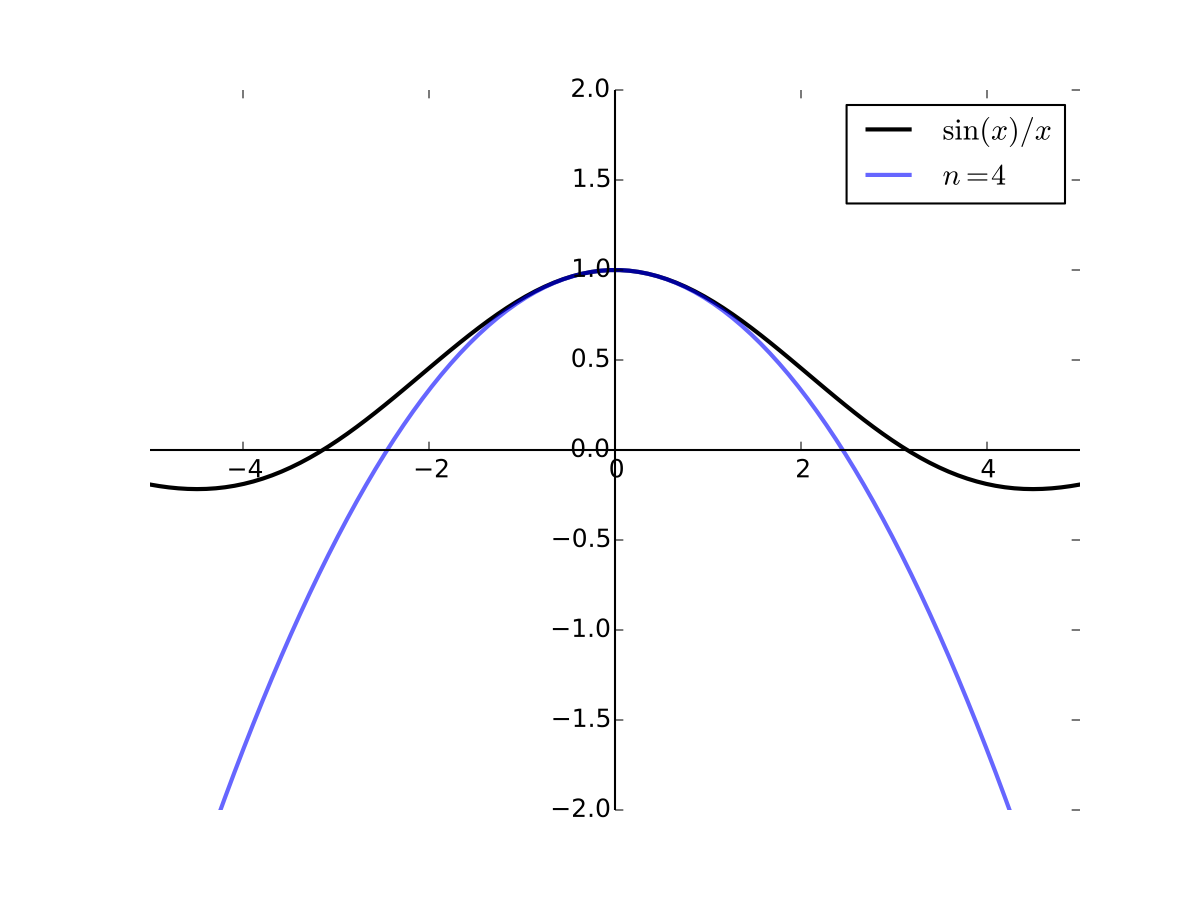
Fig. 27 4th order Taylor series for \(f(x) = \sin(x)/x\) at 0

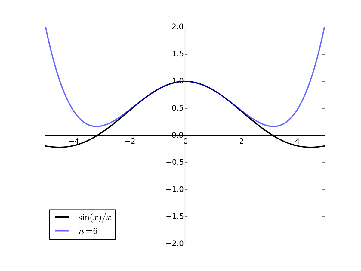
Fig. 28 6th order Taylor series for \(f(x) = \sin(x)/x\) at 0

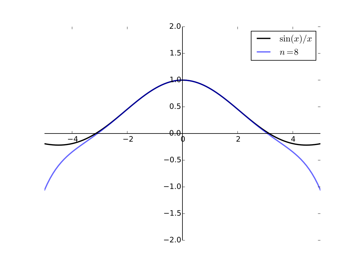
Fig. 29 8th order Taylor series for \(f(x) = \sin(x)/x\) at 0

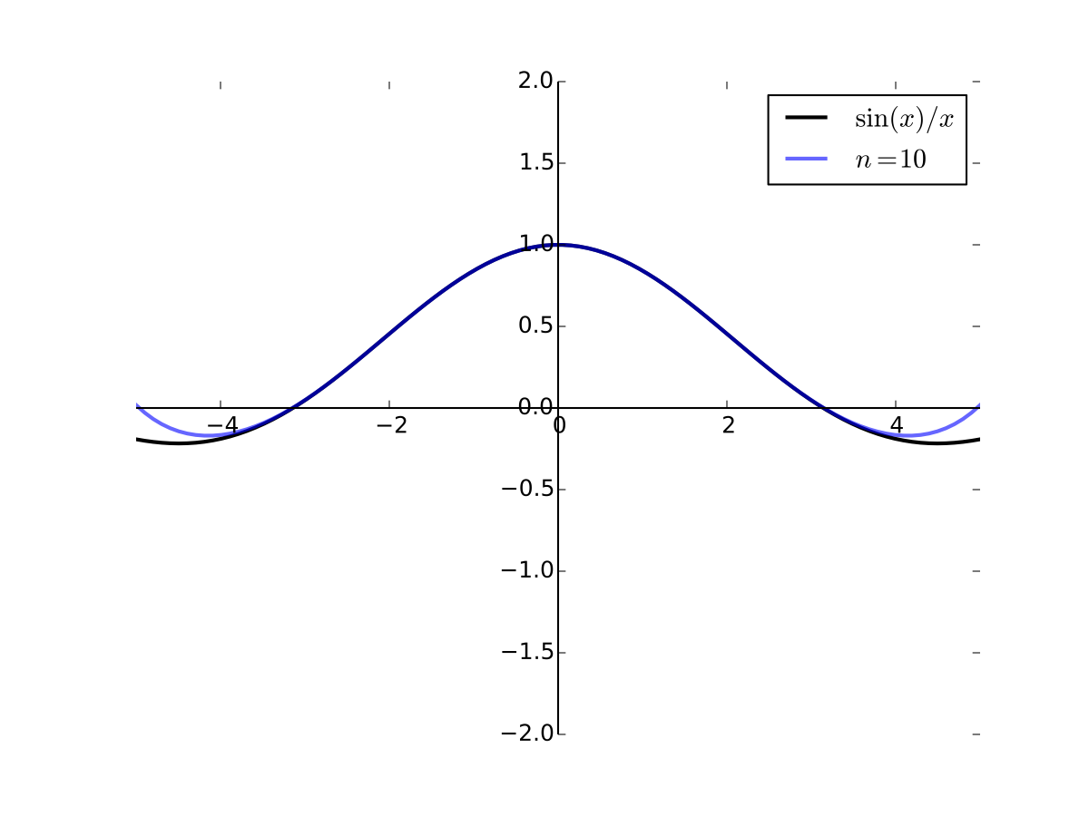
Fig. 30 10th order Taylor series for \(f(x) = \sin(x)/x\) at 0

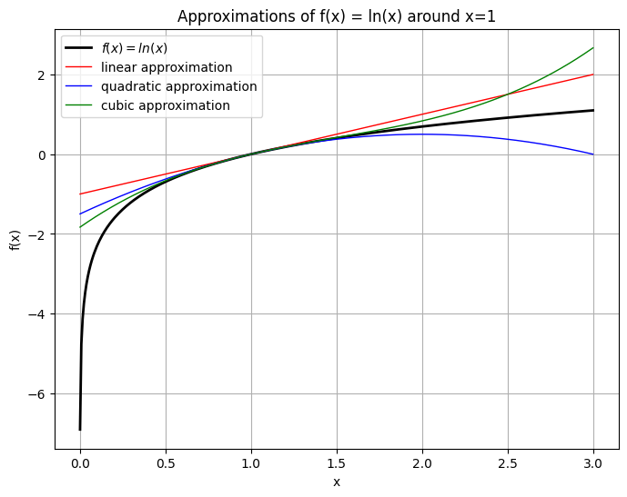
Example

Consider function \(f(x) = \ln(x)\) and let \(a=1\). Let’s approximate \(f(x)\) with Taylor series at \(a=1\).

Not that \(f'(x) = 1/x\), \(f''(x) = -1/x^2\), \(f'''(x) = 2/x^3\)

Linear approximation:

\[ f(x) = f(a) + f'(a)(x-1) = f(1) + f'(1)(x-1) = 0 + 1(x-1) = x-1 \]

Quadratic approximation:

\[\begin{split} f(x) = f(a) + f'(a)(x-1) + \frac{f''(a)}{2}(x-1)^2 = \\ 0 + 1(x-1) - \frac{1}{2}(x-1)^2 = \\ x-1 - \frac{1}{2}(x^2 - 2x + 1) = \\ -\frac{1}{2}x^2 + 2x - \frac{3}{2} \end{split}\]

Quadratic approximation:

\[\begin{split} f(x) = f(a) + f'(a)(x-1) + \frac{f''(a)}{2}(x-1)^2 + \frac{f'''(a)}{2 \cdot 3}(x-1)^3 = \\ 0 + 1(x-1) - \frac{1}{2}(x-1)^2 + \frac{1}{3}(x-1)^3 = \\ x-1 - \frac{1}{2}(x^2 - 2x + 1) + \frac{1}{3}(x^3 - 3x^2 + 3x - 1) = \\ \frac{1}{3}x^3 -\frac{3}{2}x^2 + 3x - \frac{11}{6} \end{split}\]

Show code cell source Hide code cell source

import numpy as np
import matplotlib.pyplot as plt

# Generate x values for the plot
x_vals = np.linspace(0.001, 3, 400)
y1_vals = np.log(x_vals)
y2_vals = x_vals-1
y3_vals = -1.5 + 2*x_vals - 0.5*x_vals**2
y4_vals = x_vals**3/3 -1.5*x_vals**2 + 3*x_vals - 11/6

plt.figure(figsize=(8, 6))

plt.plot(x_vals, y1_vals, label=r'$f(x) = ln(x)$', color='black', linewidth=2)
plt.plot(x_vals, y2_vals, label=r'linear approximation', color='red', linewidth=1)
plt.plot(x_vals, y3_vals, label=r'quadratic approximation', color='blue', linewidth=1)
plt.plot(x_vals, y4_vals, label=r'cubic approximation', color='green', linewidth=1)

# Labels and legend
plt.xlabel('x')
plt.ylabel('f(x)')
plt.title('Approximations of f(x) = ln(x) around x=1')
plt.legend()
plt.grid(True)
plt.show()