📖 Bivariate optimization

⏱ | words

References and additional materials

[Sydsæter, Hammond, Strøm, and Carvajal, 2016]

Chapter 13.1-13.3

[Sydsæter, Hammond, Strøm, and Carvajal, 2016]

The rest of chapter 13 can be used as additional reading material for further study, also see Chapter 14 for more advanced constrained optimization method.

Maximizers and minimizers

The foundations of optimization are the same as in one dimension, but the optimum criteria differ in important ways.

Please, review optimization of univariate functions beforehand.

Definition

Consider \(f \colon A \to \mathbb{R}\) where \(A \subset \mathbb{R}^2\).

A point \((x_1^*, x_2^*) \in A\) is called a (global) maximizer of \(f\) on \(A\) if

\[ f(x_1^*, x_2^*) \geq f(x_1, x_2) \quad \text{for all} \quad (x_1, x_2) \in A \]

A point \((x_1^*, x_2^*) \in A\) is called a (global) minimizer of \(f\) on \(A\) if

\[ f(x_1^*, x_2^*) \leqslant f(x_1, x_2) \quad \text{for all} \quad (x_1, x_2) \in A \]

We will briefly consider both the unconstrained and constrained optimization problems:

• Unconstrained: assume that \(A\) is the entire space \(\mathbb{R}^2\) or at least the entire domain of function \(f\)

• Constrained: \(A\) is defined by some constraints, and so the task is to maximize or minimize \(f(x_1, x_2)\) subject to these constraints

It is also important to keep in mind the destinction between global and local maximizers and minimizers:

• The definition above refers to global maximizers and minimizers

• The optimal criteria below refer merely to the local maximizers and minimizers

It is sometimes possible to reconcile the two optima by directly comparing the value of the objective function \(f\) at all found local optima and choose the one with the highest value.

Definition

Consider a function \(f: A \to \mathbb{R}\) where \(A \subset \mathbb{R}^n\). A point \(x^* \in A\) is called a

• local maximizer of \(f\) if \(\exists \delta>0\) such that \(f(x^*) \geq f(x)\) for all \(x \in B_\delta(x^*) \cap A\)

• local minimizer of \(f\) if \(\exists \delta>0\) such taht \(f(x^*) \leq f(x)\) for all \(x \in B_\delta(x^*) \cap A\),

where \(B_\delta(x^*)\) is the open ball of radius \(\delta\) centered at \(x^*\), i.e.

\[ B_\delta(x^*) = \{x \in \mathbb{R}^n: ||x - x^*|| < \delta\} \]

In other words, a local optimizer is a point that is a maximizer/minimizer in some neighborhood of it and not necesserily in the whole function domain.

First order conditions

Similar to the univariate case, the first order conditions (FOCs) are based on the first order derivatives of the function \(f\).

It’s important to remember that the first order conditions come in two flavors:

• Necessary FOCs: these are conditions that must be satisfied when we already have a point which is known to be a maximizer or minimizer

• Sufficient FOCs: these are conditions that, if satisfied, guarantee that a point is a maximizer or minimizer

Necessary first order conditions

When they exist, denote the partial derivatives at \((x_1, x_2) \in A\) as

\[\begin{split} f'_1(x_1, x_2) = \frac{\partial f(x_1, x_2)}{\partial x_1} \\ f'_2(x_1, x_2) = \frac{\partial f(x_1, x_2)}{\partial x_2} \end{split}\]

Definition

An interior point \((x_1, x_2) \in A\) is called stationary for a differentiable function \(f \colon \mathbb{R}^2 \to \mathbb{R}\) if

\[ f'_1(x_1, x_2) = f'_2(x_1, x_2) = 0 \]

More generally, given a function \(f \colon \mathbb{R}^n \to \mathbb{R}\), a point \(x \in \mathbb{R}^n\) is called a stationary point of \(f\) if \(\nabla f(x) = {\bf 0}\)

• Note gradient \(\nabla f(x)\) and zero vector \({\bf 0} = (0,\dots,0)\)

Fact (Necessary FOCs)

Let \(f(x) \colon \mathbb{R}^2 \to \mathbb{R}\) be a differentiable function and let \((x_1^\star,x_2^\star)\) be an interior (local) maximizer/minimizer of \(f\). Then \(x^\star\) is a stationary point of \(f\), that is \(\nabla f(x^\star) = 0\)

\[ x^* \text{ is interior maximizer/minimizer } \implies \nabla f(x^\star) = {\bf 0} \]

Example

\[ f(x_1, x_2) = x_1^2 + 4 x_2^2 \rightarrow \min \]

1. Compute partials and set them to zero

\[ f'_1(x_1, x_2) = 2 x_1 = 0 \quad \text{and} \quad f'_2(x_1, x_2) = 8 x_2 = 0 \]

2. Solve for stationary points: we have the unique stationary point \((0, 0)\)

3. This may be a minimizer or maximizer, but we don’t know for sure

Nasty secret 1: Solving for \((x_1, x_2)\) such that \(f'_1(x_1, x_2) = 0\) and \(f'_2(x_1, x_2) = 0\) can be hard

• System of nonlinear equations

• Might have no analytical solution

• Set of solutions can be a continuum

Example

(Don’t) try to find all stationary points of

\[ f(x_1, x_2) = \frac{\cos(x_1^2 + x_2^2) + x_1^2 + x_1}{2 + p(-x_1^2) + \sin^2(x_2)} \]

Nasty secret 2: This is only a necessary condition! We can not be sure that a found stationary point is a maximizer or minimizer.

Example

Fig. 49 Minimizer of a quadratic function \(f(x,y)=x^2+xy+2y^2\)

Fig. 50 Saddle point of a quadratic function \(f(x,y)=x^2+xy-2y^2\)

Sufficient first order conditions

Recall that in the univariate case, the shape of the function that was determined by the second order derivative played an important role.

• concave functions \(\rightarrow\) maximizers, unique if strictly concave

• convex functions \(\rightarrow\) minimizers, unique if strictly convex

How to check the shape of a bivariate function?

Write the second-order Taylor approximation for a twice-differentiable bivariate function \(f:\mathbb R^2\to\mathbb R\) at \(\boldsymbol{a} \in \mathbb R^2\), where we let \(\boldsymbol{v} = \boldsymbol{x}-\boldsymbol{a} \in \mathbb R^2\)

\[\begin{split} \begin{array}{l} f(x_1,x_2) \approx f(\boldsymbol{a}) + \nabla f(\boldsymbol{a}) \boldsymbol{v} + \frac{1}{2} \boldsymbol{v}^T Hf(\boldsymbol{a}) \boldsymbol{v} = \\ f(a_1,a_2) + \Big( f'_1(a_1,a_2), f'_2(a_1,a_2) \Big) \begin{pmatrix} x_1-a_1 \\ x_2-a_2 \end{pmatrix} + \frac{1}{2} \begin{pmatrix} x_1-a_1 \\ x_2-a_2 \end{pmatrix}^T \begin{pmatrix} f''_{11}(a_1,a_2) & f''_{12}(a_1,a_2) \\ f''_{21}(a_1,a_2) & f''_{22}(a_1,a_2)\end{pmatrix} \begin{pmatrix} x_1-a_1 \\ x_2-a_2 \end{pmatrix} \end{array} \end{split}\]

where \(f'_i = \frac{\partial f}{\partial x_i}\) and \(f''_{ij} = \frac{\partial^2 f}{\partial x_i\partial x_j}\)

The three terms in this approximation are:

1. Constant term \(f(\boldsymbol{a})\) defines the over level of the approximation

2. Linear term \(\nabla f(\boldsymbol{a})\cdot(\boldsymbol{x}-\boldsymbol{a})\) reflects the slope of the function

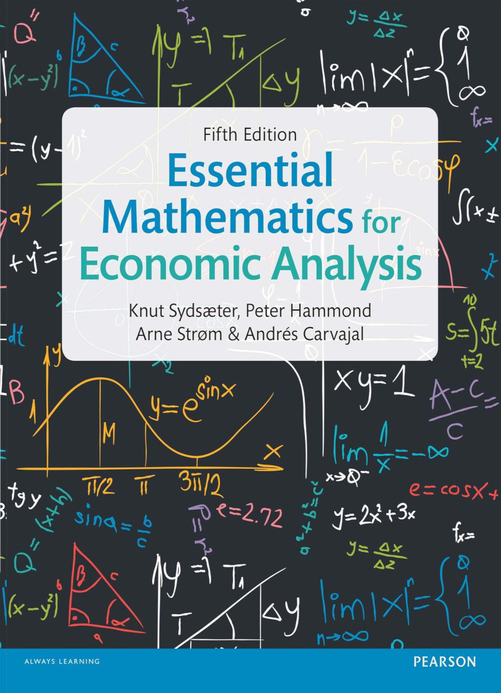
3. Quadratic term \((\boldsymbol{x}-\boldsymbol{a})^T \cdot Hf(\boldsymbol{a})\cdot (\boldsymbol{x}-\boldsymbol{a})\) defines the shape of the function

There are three general shapes of the general quadratic function

\[ f(\boldsymbol{x}) = \boldsymbol{x}^T A \boldsymbol{x}, \; \text{where} \; A \; \text{is a symmetric matrix}, \]

which is referred to as a quadratic form.

In our case, \(A\) is a Hessian matrix of the function (symmetric by Young’s theorem!), and we are interested in the values of the quadratic form at the point \(\boldsymbol{x} - \boldsymbol{a}\).

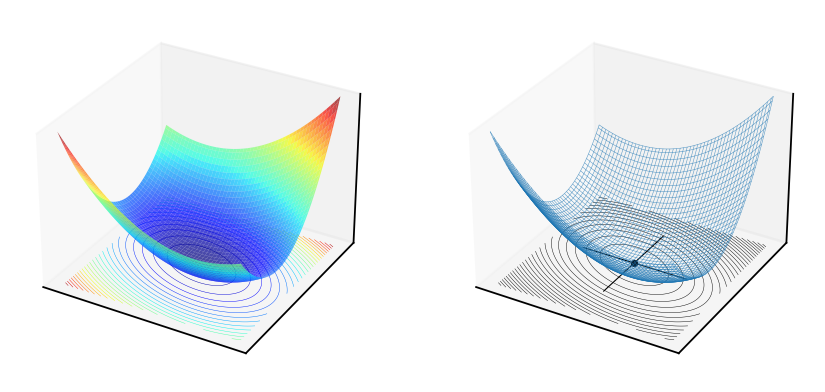
Fig. 51 Convex quadratic form \(f(x,y)=x^2+xy+2y^2\), \(A = \begin{pmatrix} 1 & \tfrac{1}{2} \\ \tfrac{1}{2} & 2 \end{pmatrix}\)

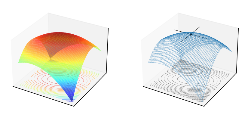
Fig. 52 Concave quadratic form \(f(x,y)=-x^2+xy-2y^2\), \(A = \begin{pmatrix} -1 & \tfrac{1}{2} \\ \tfrac{1}{2} & -2 \end{pmatrix}\)

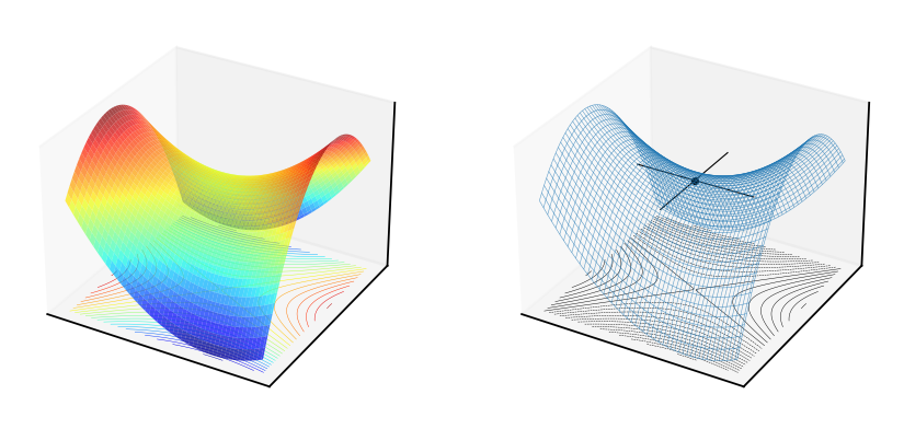
Fig. 53 Saddle point of the quadratic form \(f(x,y)=x^2+xy-2y^2\), \(A = \begin{pmatrix} 1 & \tfrac{1}{2} \\ \tfrac{1}{2} & -2 \end{pmatrix}\)

How can we tell which of the three shapes we have?

Diagonalization of quadratic forms with eigenvalues

Through the magic of linear algebra, by the change of variables \(\boldsymbol{x} \to \tilde{\boldsymbol{x}}\), we can always represent a quadratic form \(\boldsymbol{x}^T A \boldsymbol{x}\) for any symmetric \(A\) as

\[\begin{split} \boldsymbol{\tilde{x}}^T \begin{pmatrix} \lambda_1 & 0 \\ 0 & \lambda_2 \end{pmatrix} \boldsymbol{\tilde{x}} = \lambda_1 \tilde{x}_1^2 + \lambda_2 \tilde{x}_2^2 \end{split}\]

This is a direct generalization of the parabola from one dimension to two, and it is very clear whether it is concave (and thus has a maximum) of convex (and thus has a minimum)!

• recall the definitions for convexity and concavity

The general definition of convexity/concavity can be simplified when there are only three possible shapes, and expressed in the sign of the quadratic form. We have

\[ \lambda_1>0,\lambda_2>0 \implies \boldsymbol{x}^T A \boldsymbol{x}>0\,; \forall \boldsymbol{x} \neq 0,\; \text{like}\; y=x^2\;,\text{convex} \]

\[ \lambda_1<0,\lambda_2<0 \implies \boldsymbol{x}^T A \boldsymbol{x}<0\,; \forall \boldsymbol{x} \neq 0,\; \text{like}\; y=-x^2\;, \text{concave} \]

\[ \lambda_1>0,\lambda_2<0\; \text{or}\; \lambda_1<0,\lambda_2>0 \implies \text{not concave/convex, saddle point} \]

---

Values on the diagonal \(\lambda_1\) and \(\lambda_2\) are called the eigenvalues of the matrix \(A\), and satisfy the following equation for \(\lambda\), with \(I\) being the identity matrix:

\[ \det(A - \lambda I) = 0 \]

In other words, we can find \(\lambda_1\) and \(\lambda_2\) by solving the following equation:

\[\begin{split} \begin{array}{l} \det \begin{pmatrix} a_{11} - \lambda & a_{12} \\ a_{21} & a_{22}- \lambda \end{pmatrix} = 0 \\ (a_{11} - \lambda)(a_{22} - \lambda) - a_{12} a_{21} = 0 \\ \lambda^2 - \lambda a_{22} - \lambda a_{11} + a_{11} a_{22} - a_{12} a_{21} = 0 \\ \lambda^2 - \mathrm{trace}(A)\lambda + \det(A) = 0 \\ \end{array} \end{split}\]

Hence the the two eigenvalues \(\lambda_1\) and \(\lambda_2\) of \(A\) are given by the two roots of

\[ \lambda^2 - \mathrm{trace}(A) \lambda + \det(A) = 0 \]

From the Viets’s formulas for a quadratic polynomial we have

\[\begin{split} \lambda_1 + \lambda_2 = \mathrm{trace}(A) \\ \lambda_1 \lambda_2 = \mathrm{det}(A) \end{split}\]

We can now formulate the Hessian based shape criterion and sufficient first order conditions.

Fact

If \(f \colon \mathbb{R}^2 \to \mathbb{R}\) is a twice continuously differentiable function, then

1. \(\det\big(Hf(x)\big) \geqslant 0\) and \(\mathrm{trace}\big(Hf(x)\big)\geqslant0\) for all \(x\) \(\implies\) both eigenvalues are non-negative \(\implies f\) (weakly) convex

2. \(\det\big(Hf(x)\big) \geqslant 0\) and \(\mathrm{trace}\big(Hf(x)\big)\leqslant0\) for all \(x\) \(\implies\) both eigenvalues are non-positive \(\implies f\) (weakly) concave

3. \(\det\big(Hf(x)\big)>0\) and \(\mathrm{trace}\big(Hf(x)\big)>0\) for all \(x\) \(\implies\) both eigenvalues are positive \(\implies f\) strictly convex

4. \(\det\big(Hf(x)\big)>0\) and \(\mathrm{trace}\big(Hf(x)\big)<0\) for all \(x\) \(\implies\) both eigenvalues are negative \(\implies f\) strictly concave

Fact (sufficient FOCs)

Let \(f \colon \mathbb{R}^2 \to \mathbb{R}\) be concave/convex differentiable function. Then \(x^*\) is a minimizer/minimizer of \(f\) if and only if \(x^*\) is a stationary point of \(f\).

\[ f \text{ concave } \implies \nabla f(x^*) = 0 \iff x^* \text{ is maximizer } \]

\[ f \text{ convex } \implies \nabla f(x^*) = 0 \iff x^* \text{ is minimizer } \]

• Note that the function \(f\) is assumed to have domain equal to \(\mathbb{R}^2\), otherwise there are additional conditions on its domain (it has to be a convex set) and the stationary point (it has to be an interior point of the domain)

Fact (sufficient conditions for uniqueness)

Let \(f \colon \mathbb{R}^2 \to \mathbb{R}\) be strictly concave/convex differentiable function, and let \(x^*\) be a stationary point. Then \(x^*\) is the unique minimizer/maximizer of \(f\).

\[ f \text{ strictly concave } \implies \nabla f(x^*) = 0 \iff x^* \text{ is unique maximizer } \]

\[ f \text{ strictly convex } \implies \nabla f(x^*) = 0 \iff x^* \text{ is unique minimizer } \]

Example

Let \(A := (0, \infty) \times (0, \infty)\) and let \(U \colon A \to \mathbb{R}\) be the utility function

\[ % U(c_1, c_2) = \alpha \ln c_1 + \beta \ln c_2 % \]

We assume that \(\alpha\) and \(\beta\) are both strictly positive, and assume that all required conditions on \(A\) mentioned above are satisfied.

The gradient and the Hessian of the function \(U\) are given by

\[ \nabla U(c_1, c_2) = \begin{pmatrix} \frac{\partial U}{\partial c_1} & \frac{\partial U}{\partial c_2} \end{pmatrix} = \begin{pmatrix} \frac{\alpha}{c_1} & \frac{\beta}{c_2} \end{pmatrix} \]

\[\begin{split} HU(c_1, c_2) = \begin{pmatrix} \frac{\partial^2 U}{\partial c_1^2} & \frac{\partial^2 U}{\partial c_1 \partial c_2} \\ \frac{\partial^2 U}{\partial c_2 \partial c_1} & \frac{\partial^2 U}{\partial c_2^2} \end{pmatrix} = \begin{pmatrix} -\frac{\alpha}{c_1^2} & 0 \\ 0 & -\frac{\beta}{c_2^2} \end{pmatrix} \end{split}\]

We have \(\mathrm{trace}(HU) = - \left( \frac{\alpha}{c_1^2} + \frac{\beta}{c_2^2} \right) < 0\) and \(\det(HU) = \frac{\alpha \beta}{c_1^2 c_2^2} > 0\) for all \((c_1, c_2) \in A\). Thus, the function \(U\) is strictly concave on \(A\).

Exercise: What about the stationary point that would be a unique maximizer of \(U\)?

Example: unconstrained maximization of quadratic utility

\[ u(x_1, x_2) = - (x_1 - b_1)^2 - (x_2 - b_2)^2 \rightarrow \max_{x_1, x_2} \]

Intuitively the solution should be \(x_1^*=b_1\) and \(x_2^*=b_2\) to minimize quadratic loss, let’s see if the analysis leads to the same conclusion.

First, let’s find first and second derivatives of the function \(u\):

\[ \frac{\partial u(x_1, x_2)}{\partial x_1} = -2 (x_1 - b_1), \quad \frac{\partial u(x_1, x_2)}{\partial x_2} = -2 (x_2 - b_2) \]

\[ \frac{\partial^2 u(x_1, x_2)}{\partial x_1 \partial x_1} = -2, \quad \frac{\partial^2 u(x_1, x_2)}{\partial x_2 \partial x_1} = 0 \]

\[ \frac{\partial^2 u(x_1, x_2)}{\partial x_2 \partial x_1} = 0, \quad \frac{\partial^2 u(x_1, x_2)}{\partial x_2 \partial x_2} = -2 \]

\[\begin{split} \nabla u(x_1, x_2) = -2 \big( x_1 - b_1, x_2 - b_2 \big), \quad H = \begin{pmatrix} -2 & 0 \\ 0 & -2 \end{pmatrix} \end{split}\]

We have \(\mathrm{trace}(H) = -4 <0\) and \(\det(H)=4 > 0\), thus \(u(x_1,x_2)\) is strictly concave, and the FOC are sufficient for a unique maximizer.

\[ \frac{\partial}{\partial x_1} u(x_1, x_2) = -2 (x_1 - b_1) = 0 \quad \implies \quad x_1 = b_1 \]

\[ \frac{\partial}{\partial x_2} u(x_1, x_2) = -2 (x_2 - b_2) = 0 \quad \implies \quad x_2 = b_2 \]

We have found the maximizer \(x^* = (b_1, b_2)\) and have shown that it is unique, confirming our initial guess.

Second order conditions

Also come in two flavors:

• Necessary second order conditions: these are conditions that must be satisfied when we already have a point which is known to be a maximizer or minimizer

• Sufficient second order conditions: these are conditions that, if satisfied, guarantee that a point is a maximizer or minimizer

Unfortunately, there is a gap between the two sets of conditions, leaving us with a possibility of indeterminacy in some cases.

This is the complication that didn’t exist in the univariate case

Necessary second order conditions

Fact (necessary SOC)

Let \(f(x) \colon \mathbb{R}^2 \to \mathbb{R}\) be a twice continuously differentiable function and let \(x^\star \in \mathbb{R}^2\) be a local maximizer/minimizer of \(f\). Then:

• \(f\) has a local maximum at \(x^\star \in \mathbb{R}^2\) \(\implies\) \(\det\big(Hf(x^\star)\big)\geqslant 0\) and \(\mathrm{trace}\big(Hf(x^\star)\big) \leqslant 0\)

• \(f\) has a local minimum at \(x^\star \in \mathbb{R}^2\) \(\implies\) \(\det\big(Hf(x^\star)\big)\geqslant 0\) and \(\mathrm{trace}\big(Hf(x^\star)\big) \geqslant 0\)

• Note that the logical implication goes one way which is the nature of the necessary condition

We can visualize the case when strict inequality signs are replaced with the weak ones. Similar to the univariate case, the implication is that the function has flat spots, but now they can be in different dimension from the curved parts of the function

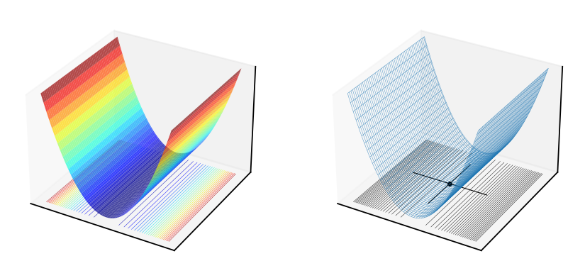
Fig. 54 Weakly convex quadratic form \(f(x,y)=x^2\) with Hessian at \((0,0)\) equal to \(H=\begin{pmatrix} 2 & 0 \\ 0 & 0 \end{pmatrix}\), \(\det(H)=0\), \(\mathrm{trace}(H)=2>0\)

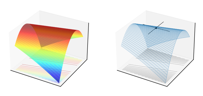
Fig. 55 [[-0.125,.5],[.5,-2]]

Weakly concave quadratic form \(f(x,y)=-0.125x^2 + xy -2y^2\) with Hessian at \((0,0)\) equal to \(H=\begin{pmatrix} -\tfrac{1}{4} & 1 \\ 1 & -4 \end{pmatrix}\), \(\det(H)=0\), \(\mathrm{trace}(H)=-4.25<0\)

• Note that in the above plots the point \((0,0)\) is a stationary point, it is local optimum — though not a unique one

Sufficient second order conditions

Fact (sufficient SOC)

Let \(f(x) \colon \mathbb{R}^2 \to \mathbb{R}\) be a twice continuously differentiable function. Then:

• if \(x\) satisfies the first order condition, \(\det\big(Hf(x^\star)\big)> 0\) and \(\mathrm{trace}\big(Hf(x^\star)\big) > 0\) is a strict local minimum of \(f\)

• if \(x\) satisfies the first order condition, \(\det\big(Hf(x^\star)\big)> 0\) and \(\mathrm{trace}\big(Hf(x^\star)\big) < 0\), then \(x^\star\) is a strict local maximum of \(f\)

\[ \nabla f(x^\star) = 0, \; \det\big(Hf(x^\star)\big)> 0 \text{ and } \mathrm{trace}\big(Hf(x^\star)\big) > 0 \implies x^\star \text{ is a strict minimum} \]

\[ \nabla f(x^\star) = 0, \; \det\big(Hf(x^\star)\big)> 0 \text{ and } \mathrm{trace}\big(Hf(x^\star)\big) < 0 \implies x^\star \text{ is a strict maximum} \]

• note again that the implication goes one way, implying that there are situation where it is impossible to determine the nature of the stationary point

• SOCs are necessary in the “weak” form, but are sufficient in the “strong” form

• this leaves room for ambiguity when we can not arrive at a conclusion — particular stationary point may be a local maximum or minimum

We can rule out saddle points: in this case when \(\det\big(Hf(x^\star)\big)<0\) but the case of \(\det\big(Hf(x^\star)\big)=0\) is not covered by any of the above conditions!

Fig. 56 Saddle point of a quadratic function \(f(x,y)=x^2+xy-2y^2\), \(\det\big(Hf(0,0)\big) = \det \begin{pmatrix} 2 & 1 \\ 1 & -4 \end{pmatrix} = -10<0\)

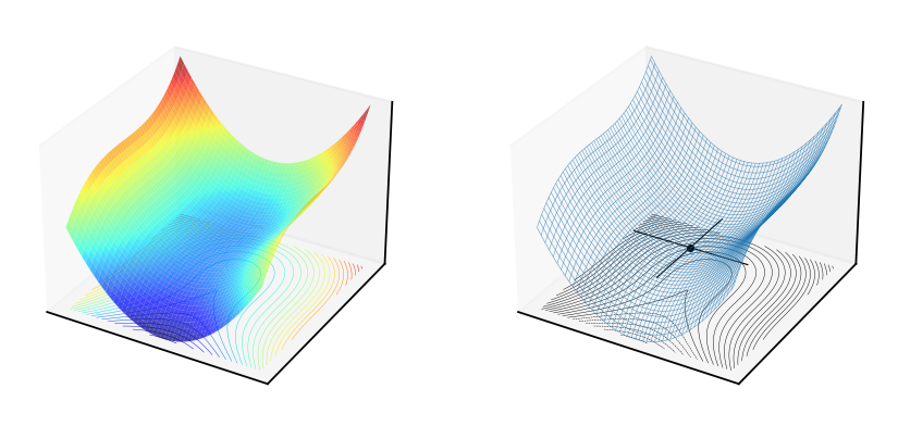
Fig. 57 Indeterminate point (not optimum) of a function \(f(x,y)=x^3+10y^2\), \(\det\big(Hf(0,0)\big) = \det \begin{pmatrix} 0 & 0 \\ 0 & 20 \end{pmatrix} = 0\)

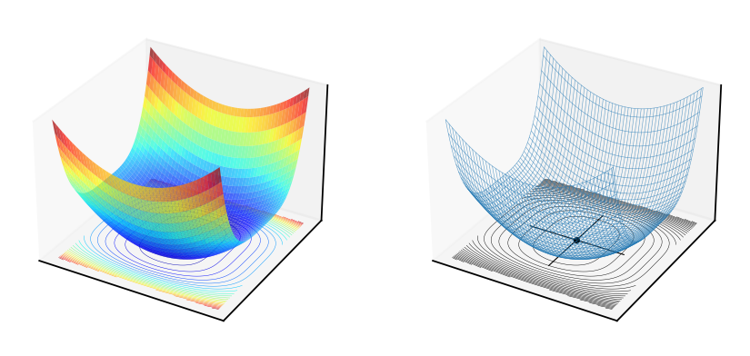
Fig. 58 Indeterminate point (yet optimum!) of a function \(f(x,y)=x^4+10y^2\), \(\det\big(Hf(0,0)\big) = \det \begin{pmatrix} 0 & 0 \\ 0 & 20 \end{pmatrix} = 0\)

Clearly, the indeterminant case of \(\det\big(Hf(x^\star)\big)=0\) can go either way, and we will only be able to conclude that the optimum is possible.

Example: Profit maximization with two inputs

\[ \pi(k, \ell) = p k^{\alpha} \ell^{\beta} - w \ell - r k \rightarrow \max_{k, \ell} \]

where \( \alpha, \beta, p, w\) are all positive and \(\alpha + \beta < 1\)

Derivatives:

• \(\pi'_1(k, \ell) = p \alpha k^{\alpha-1} \ell^{\beta} - r\)

• \(\pi'_2(k, \ell) = p \beta k^{\alpha} \ell^{\beta-1} - w\)

• \(\pi''_{11}(k, \ell) = p \alpha(\alpha-1) k^{\alpha-2} \ell^{\beta}\)

• \(\pi''_{22}(k, \ell) = p \beta(\beta-1) k^{\alpha} \ell^{\beta-2}\)

• \(\pi''_{12}(k, \ell) = p \alpha \beta k^{\alpha-1} \ell^{\beta-1}\)

First order conditions: set

\[\begin{split} \pi_1(k, \ell) = 0 \\ \pi_2(k, \ell) = 0 \end{split}\]

and solve simultaneously for \(k, \ell\) to get

\[\begin{split} k^\star = \left[ p (\alpha/r)^{1 - \beta} (\beta/w)^{\beta} \right]^{1 / (1 - \alpha - \beta)} \\ \ell^\star = \left[ p (\beta/w)^{1 - \alpha} (\alpha/r)^{\alpha} \right]^{1 / (1 - \alpha - \beta)} \end{split}\]

Exercise: Verify

Now we check second order conditions, hoping for strict inequality signs for sufficiency!

\[\begin{split} H\pi(k^\star, \ell^\star) = \begin{pmatrix} p \alpha(\alpha-1) (k^\star)^{\alpha-2} (\ell^\star)^{\beta} & p \alpha \beta (k^\star)^{\alpha-1} (\ell^\star)^{\beta-1} \\ p \alpha \beta (k^\star)^{\alpha-1} (\ell^\star)^{\beta-1} & p \beta(\beta-1) (k^\star)^{\alpha} (\ell^\star)^{\beta-2} \end{pmatrix} \end{split}\]

\[\begin{split} \begin{array}{rl} \det(H\pi(k^\star, \ell^\star)) & = \Big[\alpha(\alpha-1)\beta(\beta-1)- \alpha^2\beta^2\Big] \Big[p(k^\star)^{\alpha-1} (\ell^\star)^{\beta-1}\Big]^2 = \\ & = \alpha \beta \big(1- \alpha - \beta\big) \Big[p(k^\star)^{\alpha-1} (\ell^\star)^{\beta-1}\Big]^2 \end{array} \end{split}\]

Clearly, for \(\alpha + \beta < 1\) we have \(\det(H\pi(k^\star, \ell^\star)) > 0\).

It is also straightforward to show that the trace of the Hessian is negative when \(\alpha + \beta < 1\)

Exercise: Verify

Thus, by sufficient second order conditions, we have that \(k^\star\) and \(\ell^\star\) are unique maximizers of the profit function.

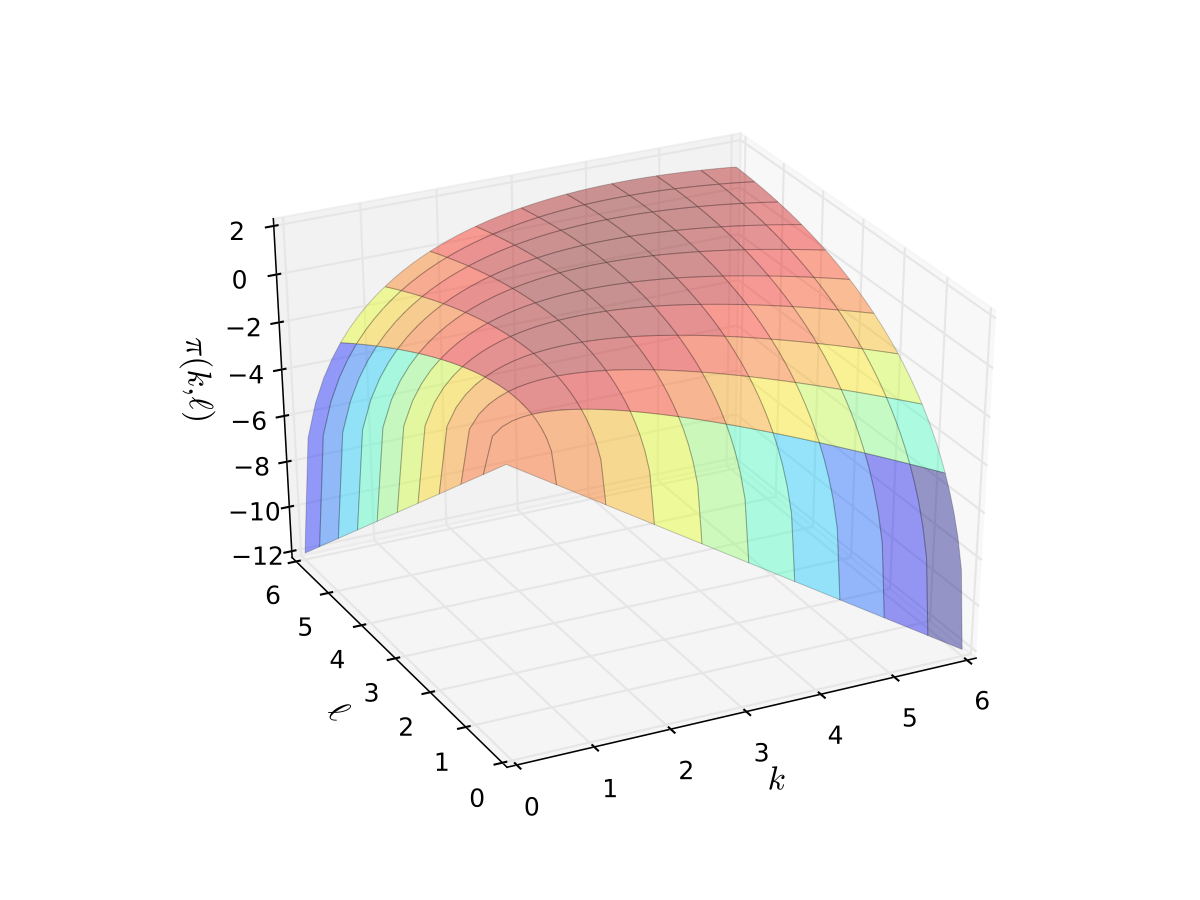
Fig. 59 Profit function when \(p=5\), \(r=w=2\), \(\alpha=0.4\), \(\beta=0.5\)

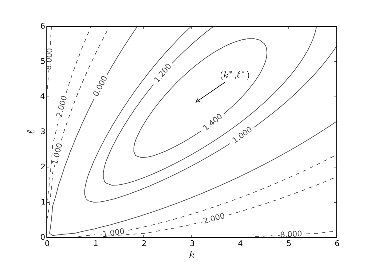
Fig. 60 Optimal choice, \(p=5\), \(r=w=2\), \(\alpha=0.4\), \(\beta=0.5\)

Simple constrained optimization

We will not consider the main method for constrained optimization, which is the Lagrange multiplier method.

Instead, look at a couple of simpler approaches that are still useful in economic applications.

We essentially take this by example, without formulating the general theory. It is much more involved, and is the subject of a separate Optimization course (ECON6012).

Constrained optimization is economics: the optimal allocation of scarce resources

• optimal = optimization

• scarce = constrained

Standard constrained problems:

• Maximize utility given budget

• Maximize portfolio return given risk constraints

• Minimize cost given output requirement

Example

Maximization of utility subject to budget constraint

\[ % \max u(x_1, x_2) \; \text{ such that } \; p_1 x_1 + p_2 x_2 \leq m % \]

• \(p_i\) is the price of good \(i\), assumed \(> 0\)

• \(m\) is the budget, assumed \(> 0\)

• \(x_i \geq 0\) for \(i = 1,2\)

• let \(u(x_1, x_2) = \alpha \log(x_1) + \beta \log(x_2)\), \(\alpha>0\), \(\beta>0\)

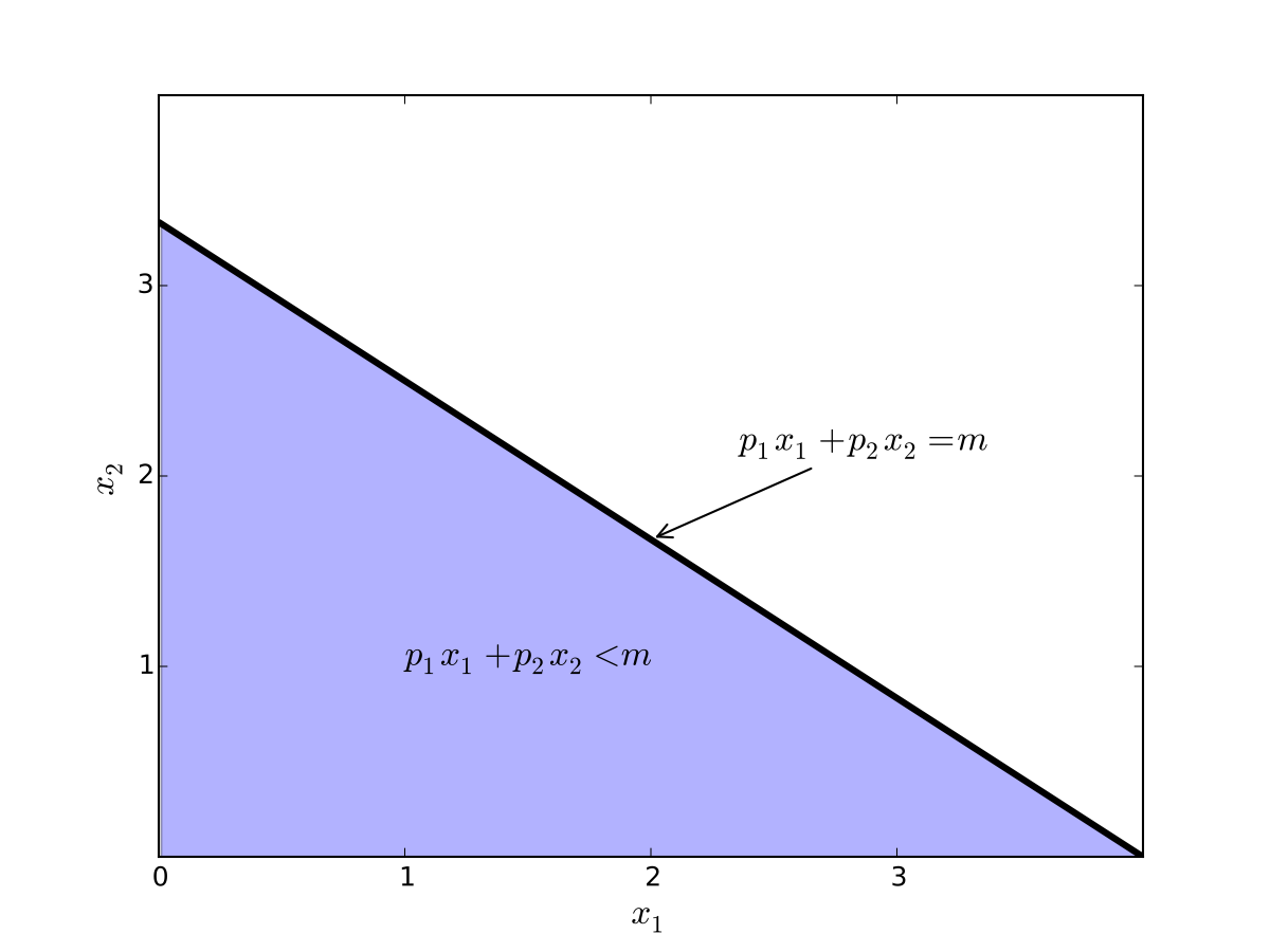
Fig. 61 Budget set when, \(p_1=0.8\), \(p_2 = 1.2\), \(m=4\)

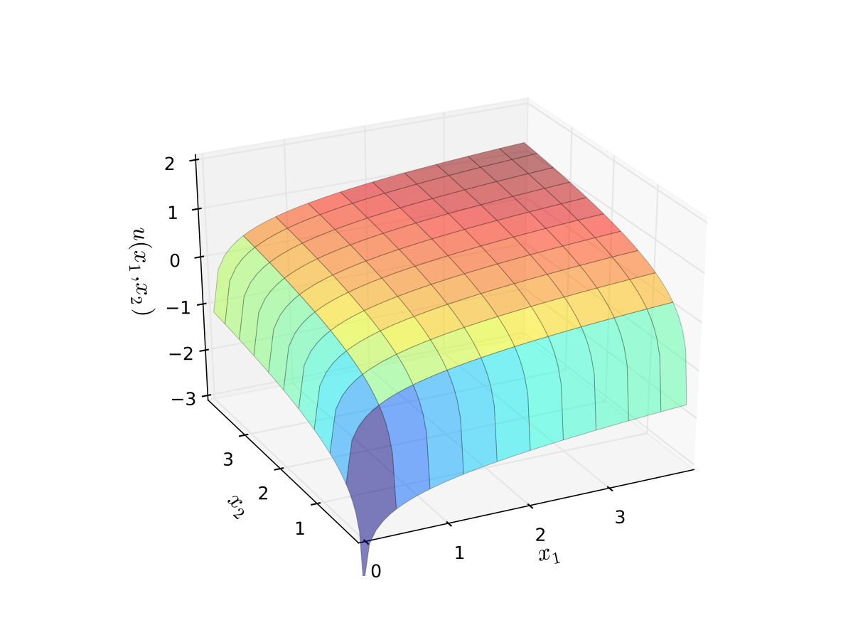
Fig. 62 Log utility with \(\alpha=0.4\), \(\beta=0.5\)

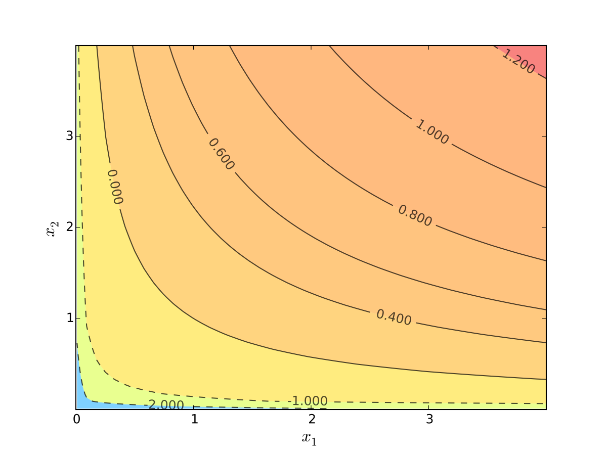
Fig. 63 Log utility with \(\alpha=0.4\), \(\beta=0.5\)

We seek a bundle \((x_1^\star, x_2^\star)\) that maximizes \(u\) over the budget set

That is,

\[ % \alpha \log(x_1^\star) + \beta \log(x_2^\star) \geq \alpha \log(x_1) + \beta \log(x_2) % \]

for all \((x_1, x_2)\) satisfying \(x_i \geq 0\) for each \(i\) and

\[ % p_1 x_1 + p_2 x_2 \leq m % \]

Visually, here is the budget set and objective function:

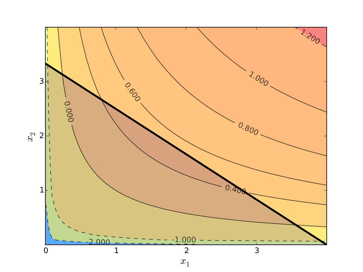
Fig. 64 Utility max for \(p_1=1\), \(p_2 = 1.2\), \(m=4\), \(\alpha=0.4\), \(\beta=0.5\)

First observation: \(u(0, x_2) = u(x_1, 0) = u(0, 0) = -\infty\)

• Hence we need consider only strictly positive bundles

Second observation: \(u(x_1, x_2)\) is strictly increasing in both \(x_i\)

• Never choose a point \((x_1, x_2)\) with \(p_1 x_1 + p_2 x_2 < m\)

• Otherwise can increase \(u(x_1, x_2)\) by small change

Hence we can replace \(\leq\) with \(=\) in the constraint

\[ % p_1 x_1 + p_2 x_2 \leq m \quad \text{becomes} \quad p_1 x_1 + p_2 x_2 = m % \]

Implication: Just search along the budget line

Substitution method

Substitute constraint into objective function and treat the problem as unconstrained

This changes

\[ % \max_{x_1, x_2} \left\{ \alpha \log(x_1) + \beta \log(x_2) \right\} \text{ such that } \; p_1 x_1 + p_2 x_2 = m % \]

into

\[ % \max_{x_1} \left\{ \alpha \log(x_1) + \beta \log((m - p_1x_1) / p_2) \right\} % \]

Since all candidates satisfy \(x_1 > 0\) and \(x_2 > 0\), the domain is

\[ 0 < x_1 < \frac{m}{p_1} \]

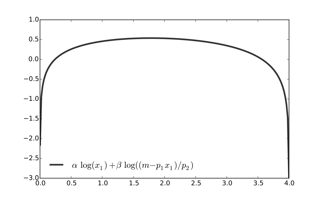
Fig. 65 Utility max for \(p_1=1\), \(p_2 = 1.2\), \(m=4\), \(\alpha=0.4\), \(\beta=0.5\)

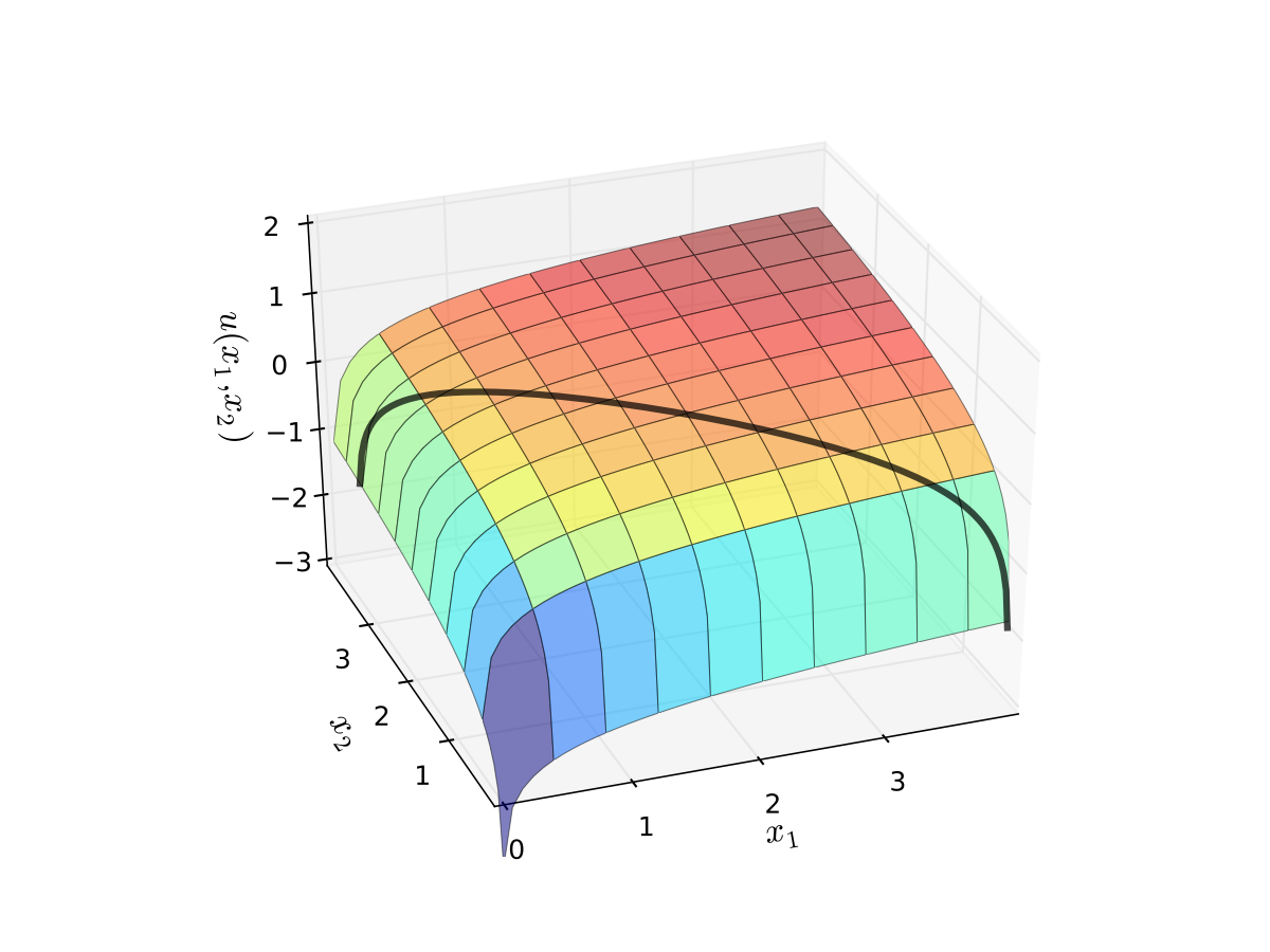
Fig. 66 Utility max for \(p_1=1\), \(p_2 = 1.2\), \(m=4\), \(\alpha=0.4\), \(\beta=0.5\)

First order condition for

\[ % \max_{x_1} \left\{ \alpha \log(x_1) + \beta \log((m - p_1x_1) / p_2) \right\} % \]

gives

\[ % x_1^\star = \frac{\alpha}{\alpha + \beta} \cdot \frac{m}{p_1} % \]

Exercise: Verify

Exercise: Check second order condition (strict concavity)

Substituting into \(p_1 x_1^\star + p_2 x_2^\star = m\) gives

\[ % x_2^\star = \frac{\beta}{\beta + \alpha} \cdot \frac{m}{p_2} % \]

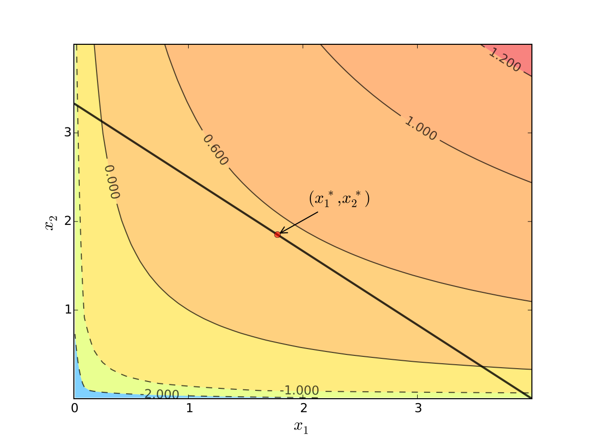
Fig. 67 Maximizer for \(p_1=1\), \(p_2 = 1.2\), \(m=4\), \(\alpha=0.4\), \(\beta=0.5\)

Substitution method: algorithm

How to solve

\[\begin{split} % \max_{x_1, x_2} \; f(x_1, x_2) \\ \text{ subject to } \\ g(x_1, x_2) = 0 % \end{split}\]

Steps:

1. Write constraint as \(x_2 = h(x_1)\) for some function \(h\)

• Solve univariate problem \(\max_{x_1} f(x_1, h(x_1))\) to get \(x_1^\star\)

9. Plug \(x_1^\star\) into \(x_2 = h(x_1)\) to get \(x_2^\star\)

Limitations:

• substitution doesn’t always work, for example for constraint \(g(x_1, x_2) = x_1^2 + x_2^2 - 1 =0\)

  • maybe we can consider sections of the constraint one-by-one: \(x_2=\sqrt{1-x_1^2}\), then \(x_2=-\sqrt{1-x_1^2}\)

• multiple constraints

  • substitute constraints one-by-one and verfity that the corresponding solution satisfies the left out constraint, in the end compare objective function values to find the best solution

  • see tutorial problem in the \(\lambda\) problem set

Tangency and relative slope conditions

Optimization approach based on tangency of contours and constraints

Example

Consider again the problem

\[\begin{split} \max_{x_1, x_2} \left\{ \alpha \log(x_1) + \beta \log(x_2) \right\} \\ \text{ such that } p_1 x_1 + p_2 x_2 = m \end{split}\]

Turns out that the maximizer has the following property:

• budget line is tangent to an indifference curve at maximizer

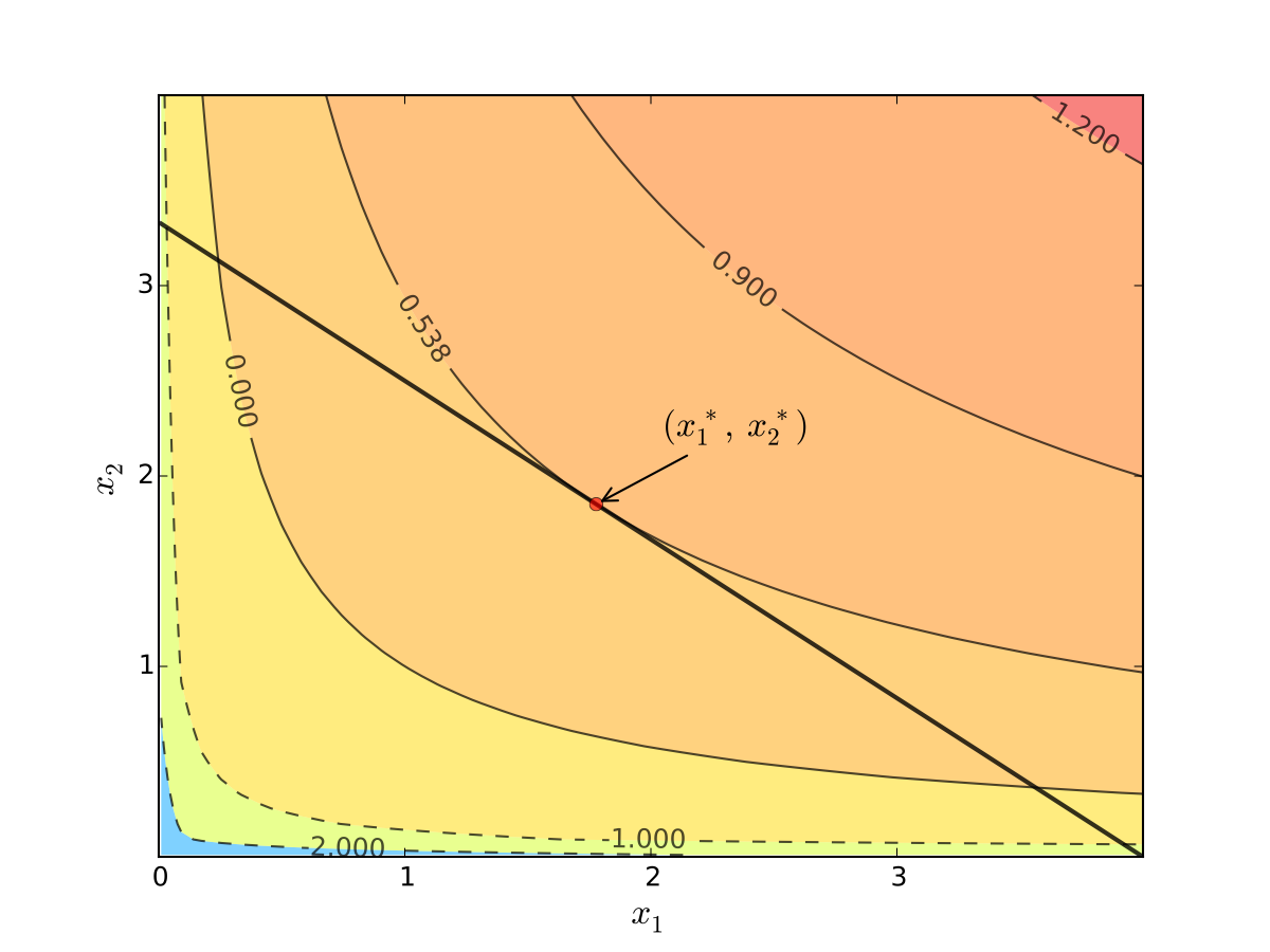
Fig. 68 Maximizer for \(p_1=1\), \(p_2 = 1.2\), \(m=4\), \(\alpha=0.4\), \(\beta=0.5\)

In fact this is an instance of a general pattern

Notation: Let’s call \((x_1, x_2)\) interior to the budget line if \(x_i > 0\) for \(i=1,2\) (not a “corner” solution, see below)

In general, any interior maximizer \((x_1^\star, x_2^\star)\) of differentiable utility function \(u\) has the property: budget line is tangent to a contour line at \((x_1^\star, x_2^\star)\)

Otherwise we can do better:

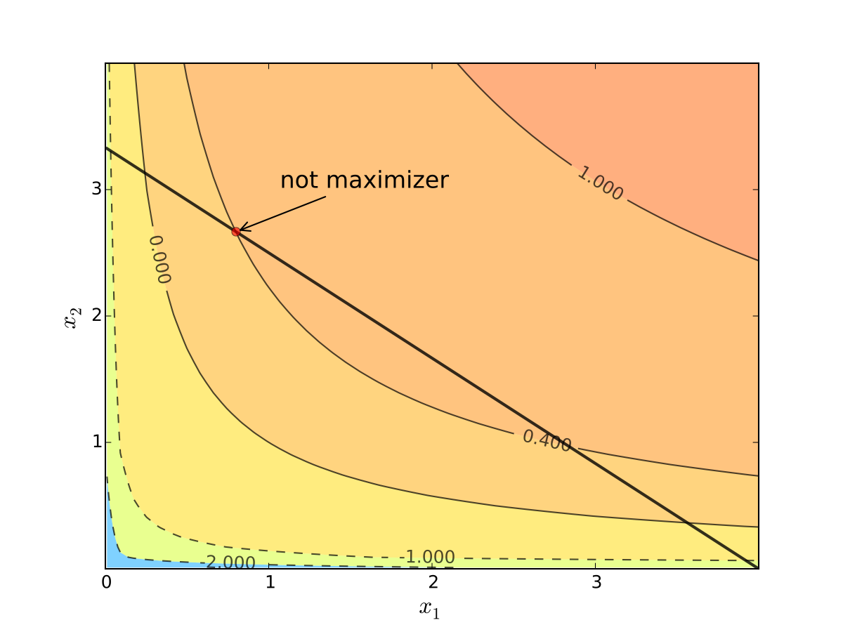
Fig. 69 When tangency fails we can do better

Necessity of tangency often rules out a lot of points

We exploit this fact to build intuition and develop more general method

Relative Slope Conditions

Consider an equality constrained optimization problem where objective and constraint functions are differentiable:

\[\begin{split} % f(x_1, x_2) \longrightarrow \max_{x_1, x_2} \\ \text{ such that } g(x_1, x_2) = 0 % \end{split}\]

How to develop necessary conditions for optima via tangency?

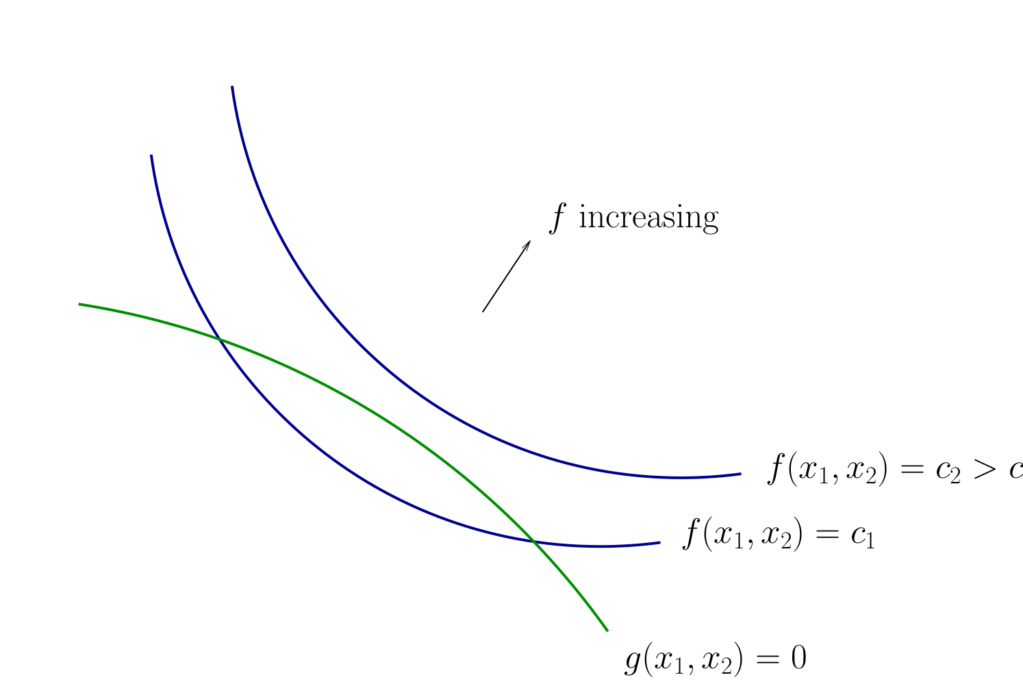
Fig. 70 Contours for \(f\) and \(g\)

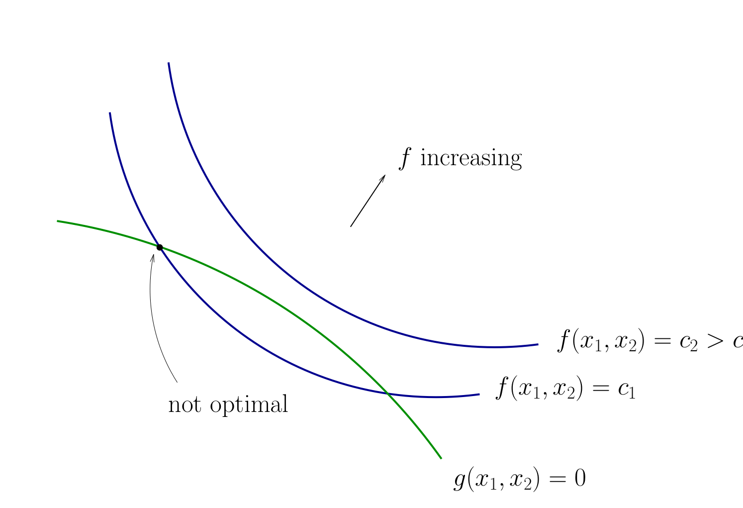
Fig. 71 Contours for \(f\) and \(g\)

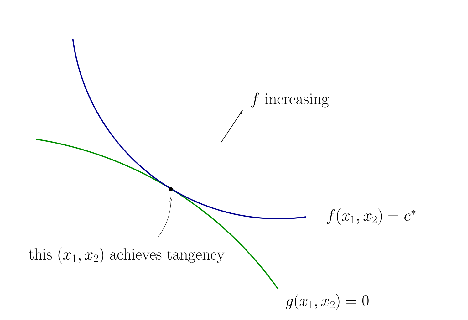
Fig. 72 Tangency necessary for optimality

How do we locate an optimal \((x_1, x_2)\) pair?

It is now good time to review the implicit functions and their derivatives!

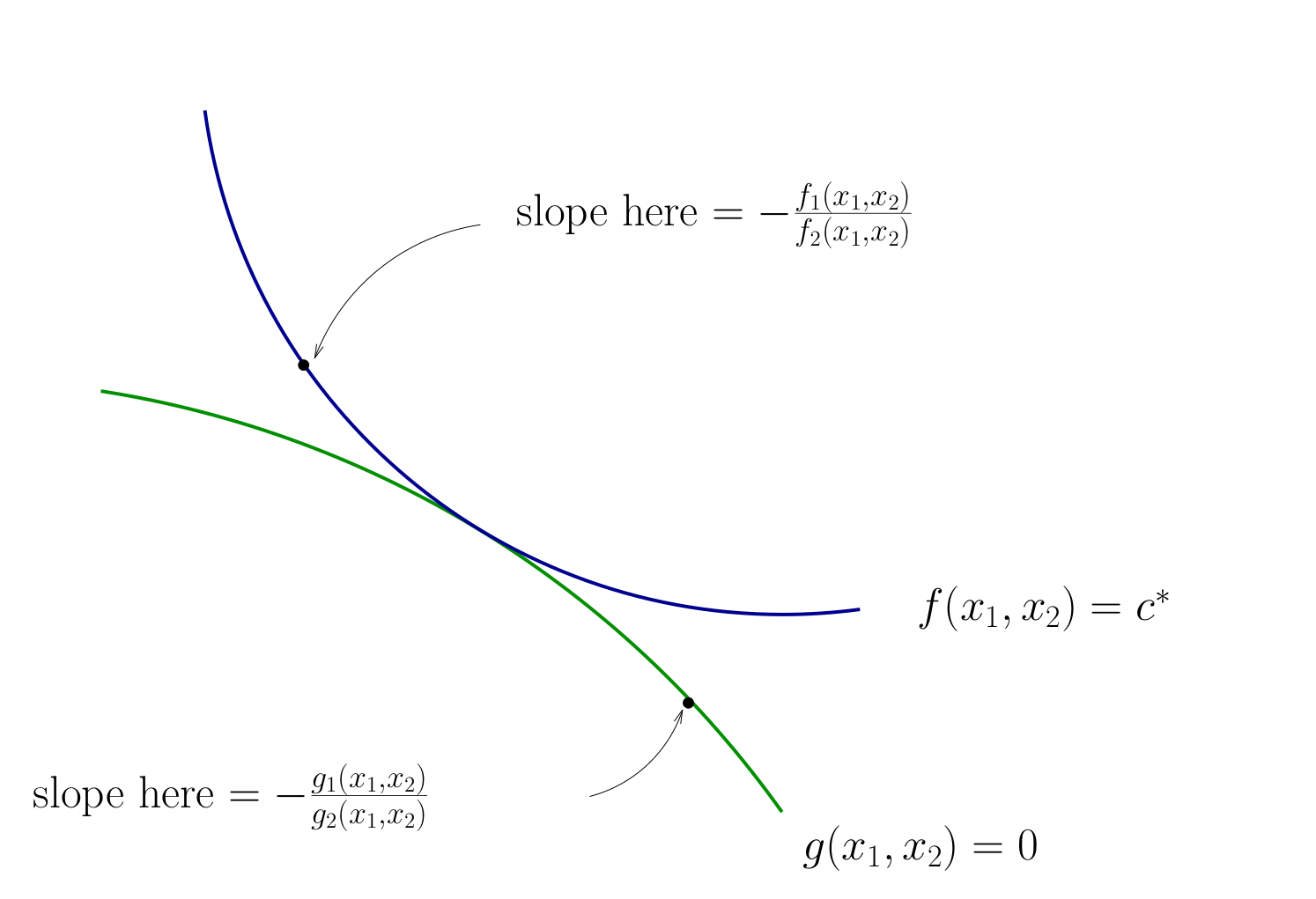
Fig. 73 Slope of contour lines

Let’s choose \((x_1, x_2)\) to equalize the slopes

That is, choose \((x_1, x_2)\) to solve

\[ % - \frac{f_1(x_1, x_2)} {f_2(x_1, x_2)} = - \frac{g_1(x_1, x_2)} {g_2(x_1, x_2)} % \]

Equivalent:

\[ % \frac{f_1(x_1, x_2)} {f_2(x_1, x_2)} = \frac{g_1(x_1, x_2)} {g_2(x_1, x_2)} % \]

Also need to respect \(g(x_1, x_2) = 0\)

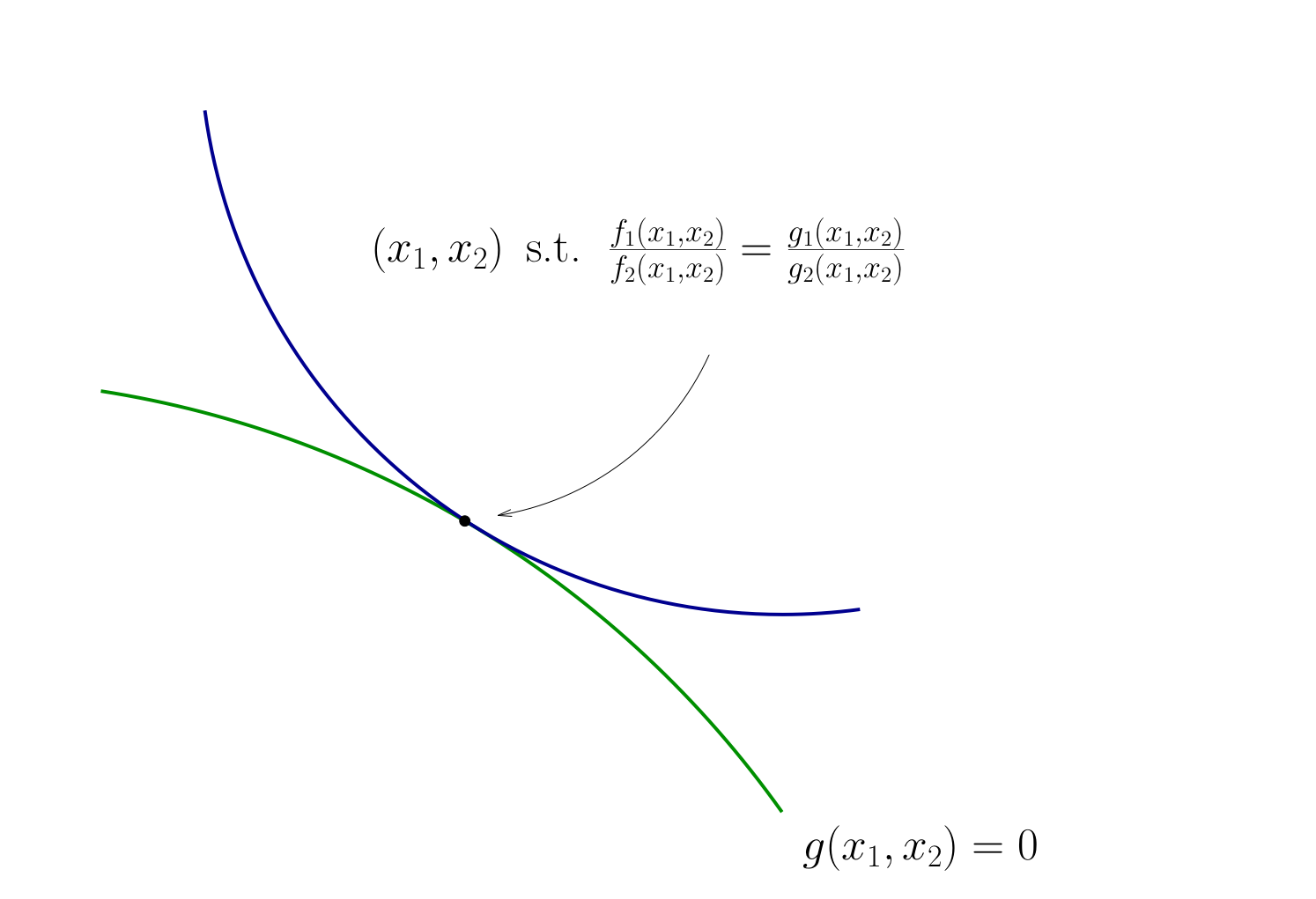
Fig. 74 Condition for tangency

Tangency conditions algorithm

In summary, when \(f\) and \(g\) are both differentiable functions, to find candidates for optima in

\[ % \max_{x_1, x_2} f(x_1, x_2) % \]

\[ % \text{ such that } \; g(x_1, x_2) = 0 % \]

1. (Impose slope tangency) Set

\[ % \frac{f_1(x_1, x_2)}{f_2(x_1, x_2)} = \frac{g_1(x_1, x_2)}{g_2(x_1, x_2)} % \]

2. (Impose constraint) Set \(g(x_1, x_2) = 0\)

3. Solve simultaneously for \((x_1, x_2)\) pairs satisfying these conditions

Example

Consider again

\[ % \max_{x_1, x_2} \left\{ \alpha \log(x_1) + \beta \log(x_2) \right\} % \]

\[ % \text{ such that } \; p_1 x_1 + p_2 x_2 - m = 0 % \]

Then

\[ % \frac{f_1(x_1, x_2)}{f_2(x_1, x_2)} = \frac{g_1(x_1, x_2)}{g_2(x_1, x_2)} \quad \iff \quad \frac{\alpha}{\beta} \frac{x_2}{x_1} = \frac{p_1}{p_2} % \]

Solving simultaneously with \(p_1 x_1 + p_2 x_2 = m\) gives

\[ % x_1^\star = \frac{\alpha}{\alpha + \beta} \cdot \frac{m}{p_1} \quad \text{and} \quad x_2^\star = \frac{\beta}{\beta + \alpha} \cdot \frac{m}{p_2} % \]

Same as before…

Limitations:

• this approach works best when you can make a diagram to have a good idea of where the optimizer will locate, especially in the case of multiple constraints

• does not work for the corner solutions where the constraint is not differentiable