🔬 Tutorial problems lambda \(\lambda\)#
Note
This problems are designed to help you practice the concepts covered in the lectures. Not all problems may be covered in the tutorial, those left out are for additional practice on your own.
\(\lambda\).1#
A critical point of a multivariate function is the point at which all partial derivatives are zero.
Compute the critical points of the following functions:
\(\quad\) \(x^4+x^2-6xy + 3y^2\)
\(\quad\) \(x^2-6xy+2y^2+10x+2y-5\)
\(\quad\) \(xy^2+x^3y-xy\)
\(\quad\) \(3x^4+3x^2y-y^3\)
\(\quad\) \(x^2+6xy+y^2-3yz+4z^2-10x-5y-21z\)
\(\quad\) \((x^2+2y^2+3z^2) e^{-(x^2+y^2+z^2)}\)
[Simon and Blume, 1994]: Exercises 17.1, 17.2
Solution algorithm:
compute partial derivatives
solve the system of equations formed by the partial derivatives equalized to zeros
Correct answers:
\((0,0), (1,1), (-1,-1)\)
\((13/7,16/7)\)
\((0,0), (0,1), (1,0), (-1,0), (1/\sqrt{5},2/5), (-1/\sqrt{5},2/5)\)
\((0,0), (1/2,-1/2), (-1/2,-1/2)\)
\((2,1,3)\)
\((0,0,0), (1,0,0), (-1,0,0), (0,1,0), (0,-1,0), (0,0,1), (0,0,-1)\)
\(\lambda\).2#
A firm uses capital and labor to produce output. When it employs \(k\) units of capital and \(\ell\) units of labor, its output is \(A k^{\alpha} \ell^{\beta}\) units, where \(A\) is a positive number, and \(\alpha + \beta < 1\).
The unit price of capital is \(r\), and the unit price of labor is \(w\); both are non-negative. The firm would like to maximize the profits taking the price \(p\) of the output as given.
The firm’s chief economist Bob presented the following formulation of the firm’s optimization problem to the CEO Alice:
Questions:
Is this formulation of the firm’s optimization problem correct?
What part reflects the revenue?
What part reflects the costs?
What are the choice variables?
Are there any constraints to be taken into account?
Right down the problem after Alice have updated the formulation.
Approach the problem as unconstrained maximization, and follow the steps in the lecture to find find all stationary points (solve the FOCs).
Write down second order partial derivatives and verify the shape conditions for the profit function.
What is the optimal strategy for the firm? Is the maximizer unique? Why?
The formulation is not correct. The revenue (after reincerting constant \(A\)) is \(p A k^{\alpha} \ell^{\beta}\), the costs are \(w \ell + r k\), and the choice variables are \(k\) and \(\ell\) (\(w\) and \(r\) are not chosen by the firm).
The constraint \(\alpha + \beta < 1\) is irrelevant for the optimization problem, instead it is a constraint on the parameters for the problem to be well posed. Relevant constraints on the optimization problem are \(k>0\) and \(\ell>0\), they can be first ignored and checked after we solve the unconstrained version of the problem.The correct formulation is (\(A, p, \alpha, \beta, w, r\) are parameters and should be fixed/found out before the firm solves the optimization problem)
See lecture notes
See lecture notes
Optimal strategy \(k^*, \ell^*\) are given in the lecture notes. The maximizer is unique because the objective function is strictly concave when \(\alpha+\beta < 1\).
Proof:
We check second order conditions for strict concavity.
What we need: for any \(k, \ell > 0\)
\(\pi_{11}(k, \ell) < 0\)
\(\pi_{11}(k, \ell) \, \pi_{22}(k, \ell) > \pi_{12}(k, \ell)^2\)
The second order derivatives are
Since \(\alpha+\beta<1\) and \(\alpha, \beta \geq 0\), we have \(\alpha-1<0\), which implies \(\pi_{11}(k,\ell)<0\) for all \(k, \ell >0\).
Moreover, the second order differentials imply
Assuming that all parameters and variables are positive. Then, we obtain \(\pi_{11}(k, \ell) \, \pi_{22}(k, \ell) > \pi_{12}(k, \ell)^2\) if and only if \((\alpha-1)(\beta-1) > \alpha \beta\) if and only if \(1 > \alpha + \beta\).
\(\lambda\).3#
An airline company has regular flights between two cities, A and B. It can treat business and pleasure travelers as separate markets by demanding advance purchase and Saturday night stay0over for pleasure travelers. Suppose that it notes a demand function of \(Q=16-p\) for business travelers and \(Q=10-p\) for pleasure travelers. Suppose also that the cost function is \(C(Q)=10+Q^2\). How much should the airline charge each type of traveler to maximize their profit? Check both first and second order conditions.
Denoting \(p_1\) the price of pleasure and \(p_2\) of business travel, the profit function is given by
The first order derivatives are given by
Checking the shape conditions, we have that
thus the profit function is concave, and the first order conditions are sufficient for a maximum. Solving for the first order conditions, we have
Solving the first equation gives us \(p_1=6\), \(p_2=14\).
\(\lambda\).4#
Imagine a consumer whose preferences are given by a utility function
over two goods \(x \geqslant 0\) and \(y\geqslant 0\) faces a limited amount of one of the goods on the market. This is reflected in an additional constraint on the feasible set of consumption bungles: in addition to a standard budget constraint, consumption of good \(x\) is limited to a maximum amount of \(\bar{x}=10\).
Together with the budget constraint the feasible set is then given by
Make a sketch of the feasible set in the \(x,y\) plane. Illustrate the interior and the corner solution.
Solve the problem by substitution method, trying in turn each of the constraints, as well their combination, if \(\alpha=1/2\). Remember to check whether the proposed solution satisfied the left out constraint.
Find the set of values of preference parameter \(\alpha\) which leads to the corner solution being optimal.
First convert the inequality constraints problem to equality by noting that the utility function is strictly increasing in each of its arguments.
Then, do not forget to consider all cases when the first, the second or both constraints are binding, as illustrated here:
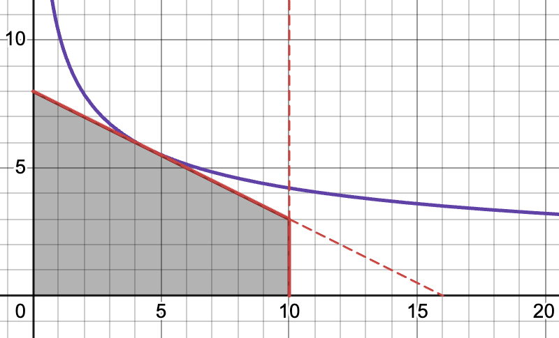
Fig. 75 Interior solution#
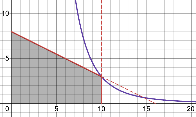
Fig. 76 Corner solution#
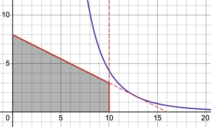
Fig. 77 Infeasible pseudo-solution you should remember to discard#
The optimization problem is given by, with \(\alpha \in (0,1) \):
We can disregard the non-negativity constraints because function \(f(x,y)\) is strictly increasing in both arguments. To see this, note that the partial derivatives of \(f(x,y)\) satisfy
for all \(x \geqslant 0\) and \(y \geqslant 0\). In other words, if we assume that an interior point \(x + 2 y < 16\), the contradiction is reached immediately because increasing either \(x\) or \(y\) towards the budget constraint increases \(f(x,y)\) compared to the initial interior point.
Effectively, the problem has two constraints, and therefore we have to consider the following cases:
Case 1. Assume that constraint \(x + 2y \leqslant 16\) is binding, i.e. \(x + 2y = 16\), and \(x = 16-2y\). Substituting this into \(f(x,y)\), we have the following univariate optimization problem
The first order condition is given by
For \(\alpha=1/2\), we have \(y=4\), \(x=8\).
It is now important to verify if the found solution satisfies the left out constraint \(x \leqslant 10\), which is true. So, point \((8,4)\) is a candidate for the optimal solution, with the corresponding utility value
Case 2. Assume that constraint \(x \leqslant 10\) is binding, i.e. \(x=10\). Plugging this into \(f(x,y)\), we have the following univariate optimization problem
It is clear that the \(\tilde{f}(y)\) is an increasing function, and therefore the written unconstrained problem has no maximum.
Case 3. Finally, assume that both constraints are binding, i.e. \(x + 2y = 16\) and \(x=10\). Then we have \(10 + 2y = 16\), or \(y=3\), that is there is only one point \((10,3)\) which satisfies both constraints. The corresponding utility value for \(\alpha=1/2\) is
Therefore, the interior solution \((8,4)\) is optimal for \(\alpha=1/2\).
We skip the second order condition check as it is not specifically asked in the problem.
To find the set of values of preference parameter \(\alpha\) which leads to the corner solution being optimal, we need to establish for which \(\alpha\) the first case holds. In other words, we want to know the last value of \(\alpha\) such that the substitution of the budget constraint holds even at the point when the second constraint becomes binding.
Recall that when the first condition is binding, we have \(y=8(1-\alpha)\) and \(x=16\alpha\). To ensure \(x \leqslant 10\) we have to require \(\alpha \leqslant \tfrac{5}{8}\).
For \(\alpha = \tfrac{5}{8}\) the budget constraint holds together with the second constraint, and for all values \(\alpha > \tfrac{5}{8}\) the solution moves beyond the constraint \(x \leqslant 10\), which is invalidates it. Thus, we can conclude that for \(\alpha > \tfrac{5}{8}\) the corner solution \((10,3)\) is optimal.