📖 Some common functions

⏱ | words

References and additional materials

[Sydsæter, Hammond, Strøm, and Carvajal, 2016]

Chapters 4.4 - 4.10

Common types of univariate functions include the following:

• Polynomial functions

  • These include constant functions, linear (and affine) functions, quadratic functions, and some power functions as special cases.

• Exponentional functions

• Power functions

• Logarithmic functions

• Trigonometric functions

  • We are unlikely to have enough time to cover trigonometric functions in this course. There are also multivariate versions of these types of functions.

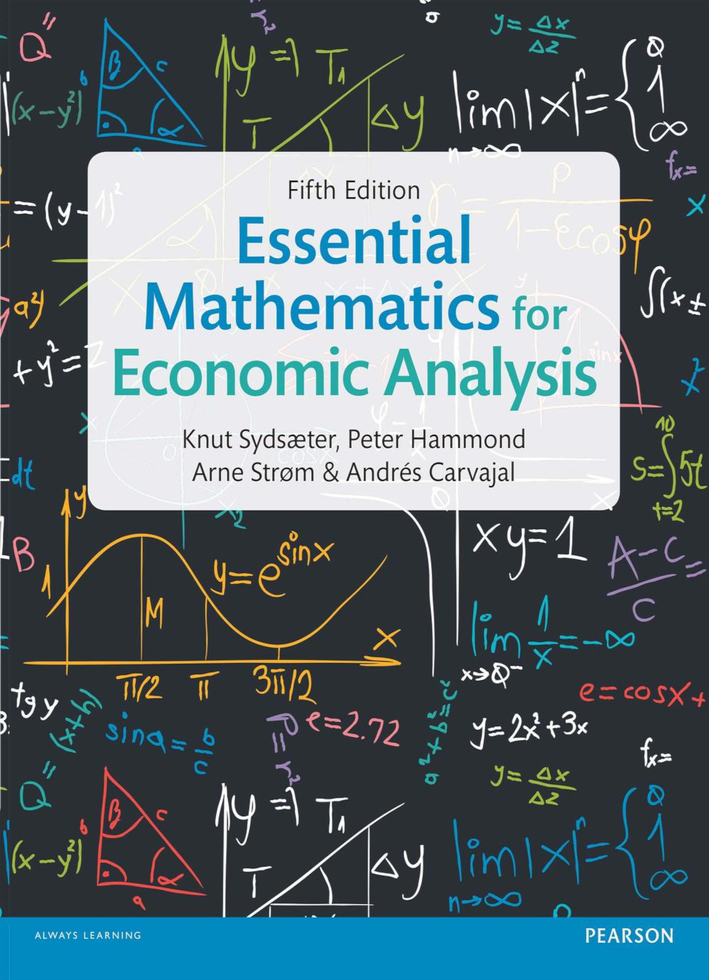
Polynomial functions

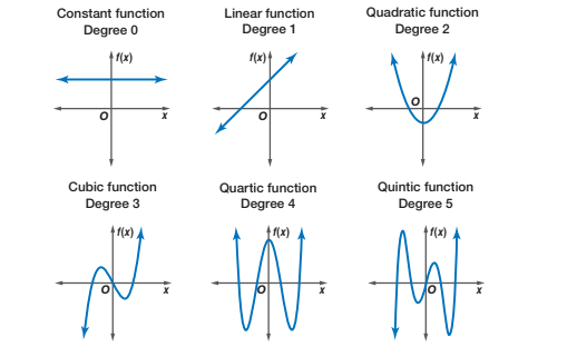
Fig. 16 Graphs of polynomial functions

Definition

A polynomial function (of one variable) is a function of the form

\[\begin{split} \begin{align*} f(x) &= \sum_{i = 0}^n a_i x^i \\ &= a_n x^n + a_{n − 1} x^{n − 1} + · · · + a_1 x^1 + a_0 x^0 \\ &= a_n x^n + a_{n − 1} x^{n − 1} + · · · + a_1 x + a_0 \end{align*} \end{split}\]

In order to distinguish between different types of polynomials, we will typically assume that the coefficient on the term with the highest power of the variable \(x\) is non-zero. The only exception is the case in which this term involves \(x^0 = 1\), in which case we will allow both \(a_0 \ne 0\) and \(a_0 = 0\).

Example

A constant (degree zero) polynomial (\(a_0 \ne 0\) or \(a_0 = 0\)):

\[ f(x) = a_0 \]

Example

A linear (degree one) polynomial (\(a_1 \ne 0\)):

\[ f(x) = a_1 x + a_0 \]

It is sometimes useful to distinguish between linear functions and affine functions.

Example

A quadratic (degree two) polynomial (\(a_2 \ne 0\)):

\[ f(x) = a_2 x^2 + a_1 x + a_0 \]

Example

A cubic (degree three) polynomial (\(a_3 \ne 0\)):

\[ f(x) = a_3 x^3 + a_2 x^2 + a_1 x + a_0 \]

Affine and linear functions

Note that strict definition of a linear function \(f(x)\) requires \(f(\alpha x) = \alpha f(x)\) and \(f(x+y) = f(x) + f(y)\), where \(\alpha, x, y \in \mathbb{R}\).

However, we often loosely speak about a linear function of one variable being a function of the form \(f(x) = a_1 x + a_0\), where \(a_0 \in \mathbb{R}\) and \(a_1 \in \mathbb{R} \setminus \{0\}\) are fixed parameters, and \(x \in \mathbb{R}\) is the single variable.

Clearly, when \(a_0 \ne 0\), the definition of a linear function is not satisfied. In fact, it satisfies a different definition, that of an affine function. Strictly speaking, linear functions are thus \(f(x) = a_1 x\), in which \(a_0 = 0\).

Using this more precise terminology, the family of linear functions is a proper subset of the family of affine functions. Note that we assume that \(a_1 \in \mathbb{R} \setminus \{0\}\) in both cases.

Exponential functions

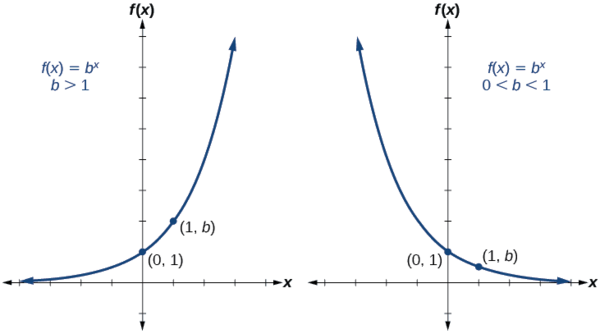
Fig. 17 Graphs of exponential functions

Definition

An exponential function is a non-linear function in which the independent variable appears as an exponent.

\[ f(x) = Ca^x \]

where \(C\) is a fixed parameter (called the coefficient), \(a \in \mathbb{R}\) is a fixed parameter (called the base), and \(x \in \mathbb{R}\) is an independent variable (called the exponent).

• Note that if \(a = 0\), then \(f(x)\) is only defined for \(x > 0\).

• Note also that if \(a < 0\), then sometimes \(f(x) \notin \mathbb{R}\). An example of this is the case when \(C = 1, a = (−1)\) and \(x = \frac{1}{2}\). In this case, we have:

\[ f(\tfrac{1}{2}) = (1)(−1)^{\frac{1}{2}} = \sqrt{−1} = i \notin \mathbb{R} \]

Popular choices of base

Two popular choices of base for exponential functions are \(a = 10\) and \(a = e\), where \(e\) denotes Euler’s constant. Euler’s constant is defined to be the number

\[ e = \lim_{n \rightarrow \infty} \left(1 + \frac{1}{n} \right)^n \]

Note that Euler’s constant is an irrational number. This means that it is a real number that cannot be represented as the ratio of an integer to a natural number.

The function \(f(x) = e^x\) is sometimes called “the” exponential function.

Exponential arithmetic

Assuming that the expressions are well-defined, we have the following laws of exponential arithmetic.

• The power of zero: \(a^0 = 1\) if \(a \ne 0\), while \(a^0\) is undefined if \(a = 0\).

• Multiplication of two exponential functions with the same base:

\[ (Ca^x)(Da^y) = CD a^{(x + y)} \]

• Division of two exponential functions with the same base:

\[ \frac{(Ca^x)}{(Da^y)} = \frac{C}{D} a^{(x - y)} \]

• An exponential function whose base is an exponential function:

\[ (Ca^x)^y = C^y a^{xy} \]

Power functions

Fig. 18 Graphs of power functions

Definition

A power function takes the form

\[ f(x) = Cx^a \]

where \(C \in \mathbb{R}\) is a fixed parameter, \(a \in \mathbb{R}\) is a fixed parameter, and \(x \in \mathbb{R}\) is an independent variable.

• Note that when \(a \in \mathbb{N}\), a power function can also be viewed as a polynomial function with a single term.

• Note that a power function can also be viewed as a type of exponential expression in which the base is \(x\) and the exponent is \(a\). This means that the laws of exponential arithmetic carry over to “power function arithmetic”.

Power function arithmetic

Assuming that the expressions are well-defined, we have the following laws of power function arithmetic.

• The power of zero: \(x^0 = 1\) if \(x \ne 0\), while \(x^0\) is undefined if \(x = 0\).

• Multiplication of two power functions with the same base:

\[ (Cx^a)(Dx^b) = CD x^{(a + b)} \]

• Division of two power functions with the same base:

\[ \frac{(Cx^a)}{(Dx^b)} = \frac{C}{D} x^{(a - b)} \]

• A power function whose base is itself a power function:

\[ (Cx^a)^b = C^b x^{ab} \]

A rectangular hyperbola

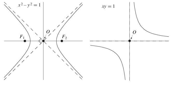
Fig. 19 Graphs of hyperbola

Consider the function \(f : \mathbb{R} \setminus \{0\} \rightarrow \mathbb{R}\) defined by \(f(x) = \frac{a}{x}\), where \(a \ne 0\). This is a special type of power function, as can be seen by noting that it can be rewritten as \(f(x) = ax^{−1}\). The equation for the graph of this function is

\[ y = \frac{a}{x} \]

Note that this equation can be rewritten as \(xy = a\). This is the equation of a rectangular hyperbola.

• Economic application: A constant “own-price elasticity of demand” demand curve.

Logarithms

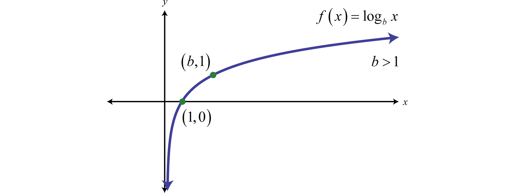
Fig. 20 Graphs of logarithmic function

Definition

A logarithm function is the inverse of an exponent.

Thus we have

\[ \log_a (a^x) = x \]

The expression \(log_a\) stands for “log base \(a\)” or “logarithm base \(a\)”. Popular choices of base are \(a = 10\) and \(a = e\).

The function

\[ g(x) = \log_a(x) \]

is the “logarithm base \(a\)” function. The “logarithm base \(a\)” function is the inverse for the “exponential base \(a\)” function. The reason for this is that

\[ g(f(x)) = g(a^x) = \log_a(a^x) = x \]

Natural (or Naperian) logarithms

A “logarithm base e” is known as a natural, or Naperian, logarithm. It is named after John Napier. See Shannon (1995, pp. 270-271) for a brief introduction to John Napier. The standard notation for a natural logarithm is \(\ln\), although you could also use \(\log_e\).

The function

\[ g(x) = \ln(x) \]

is the “logarithm base \(e\)” function. The natural logarithm function is the inverse function for “the” exponential function, since

\[ g(f(x)) = g(e^x) = \ln(e^x) = \log_e(e^x) = x \]

Illustrate the inverse (or “reflection through the 45 degree (y = x) line”) relationship between ln (x ) and ex on the whiteboard.

Logarithmic arithmetic

Assuming that the expressions are well-defined, we have the following laws of logarithmic arithmetic.

• Multiplication of two logarithmic functions with the same base:

\[ log_a(xy) = log_a(x) + log_a(y) \]

• Division of two logarithmic functions with the same base:

\[log_a \left( \frac{x}{y} \right) = log_a(x) − log_a(y) \]

• A logarithmic function whose argument is an exponential function:

\[log_a(x^y) = y \; log_a(x)\]

Note that

\[log_a(a) = log_a(a^1) = 1\]

Rational functions

Definition

A rational function \(R(x)\) is simply the ratio of two polynomial functions, \(P(x)\) and \(Q(x)\). It takes the form

\[ R(x) = \frac{P(x)}{Q(x)} = \frac{a_mx^m + a_{m−1} x^{m−1} + · · · + a_1 x + a_0} {b_n x^n + b_{n−1} x^{n−1} + · · · + b_1 x + b_0} \]

where

\[ P(x) = a_mx^m + a_{m−1} x^{m−1} + · · · + a_1 x + a_0 \]

is an \(m\)-th order polynomial (so that \(a_m \ne 0\)), and

\[ Q(x) = b_n x^n + b_{n−1} x^{n−1} + · · · + b_1 x + b_0 \]

is an \(n\)-th order polynomial (so that \(b_n \ne 0\)).

• Note that there is no requirement that the polynomial functions \(P(x)\) and \(Q(x)\) be of the same order. (In other words, we do not require that \(m = n\).)

• The most interesting case is when \(m < n\). In such cases, the rational function \(R(x)\) is called a “proper” rational function.

• When \(m > n\), then we can always use the process of long division to write the original rational function \(R(x)\) as the sum of a polynomial function \(Y(x)\) and another proper rational function \(R^∗(x)\).

Example

Consider the rational function \(R(x) = \frac{x^2 + x − 1}{x − 1}\). Note the following.

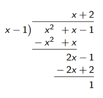
Thus we have

\[ R(x) = \frac{x^2 + x − 1}{x − 1} = (x + 2) + \left( \frac{1}{x − 1} \right) \]

Some economic examples

• Utility functions

• Production functions

• Marshallian demand functions

• Marshallian demand correspondences

• Hicksian demand functions

• Hicksian demand correspondences

• Supply functions

• Best response functions

• Best response correspondences

Utility functions

A utility function \(U : X \rightarrow \mathbb{R}\) maps a consumption set \(X\) into the real line. The consumption set \(X\) will typically be a set of possible commodity bundles or a set of possible bundles of characteristics.

Often, it will be the case that \(X = R^L_+\). Some examples include the following:

• Cobb-Douglas: \(U(x_1, x_2) = x_1^\alpha x_2^{(1 − \alpha)}\) where \(\alpha \in (0, 1)\).

• Perfect Substitutes: \(U(x_1, x_2) = x_1 + x_2\).

• Perfect Complements (or Leontief): \(U(x_1, x_2) = \text{min}(x_1, x_2)\).

Marshallian demand functions

An individual’s Marshallian demand function or correspondence \(d: \mathbb{R}^L_{++} \times \mathbb{R}_{++} \rightarrow \mathbb{R}^L_+\) maps the space of prices and income combinations into the space of commodity bundles. Example: Marshallian demands for Cobb-Douglas preferences in a two commodity world.

Here we have a Marshallian demand function:

\[ d(p_1, p_2, y) = (x_1^d (p_1, p_2, y), x_2^d(p_1, p_2, y)) = (\frac{\alpha y}{p_1}, \frac{(1 − \alpha)y}{p_2}) \]

Here we have a Marshallian demand correspondence:

\[\begin{split} d(p_1, p_2, y) = (x_1^d (p_1, p_2, y), x_2^d(p_1, p_2, y)) = \begin{cases} ( \frac{y}{p_1}, 0) \quad \text{ if } p_1 < p_2 \\ (\alpha, \frac{y − p_1 \alpha}{p_2} ) \text{ where } \alpha \in [0, \frac{y}{p_1}] \quad \text{ if } p1 = p2 \\ (0, \frac{y}{p_2}) \quad \text{ if } p_1 > p_2 \end{cases} \end{split}\]