Announcements & Reminders

• 📊 Results of the online test three

  • Average grade is 85.27 🎉

  • See distribution of grades

  • Only one test left: May 15

• 😎 Exam scheduled on Friday, May 30

📖 Functions of several variables

⏱ | words

References and additional materials

[Sydsæter, Hammond, Strøm, and Carvajal, 2016]

Chapters 11.1, 11.2, 11.3, 11.5, 12.1, 12.2, 12.3, 12.5, 12.6, 12.7

Functions of two and more variables

\[ \huge{(x_1,x_2,\dots,x_n) \in \mathbb{R}^n } \]

\[ \huge{\downarrow} \]

\[ \huge{\downarrow} \]

\[ \huge{f(x) \in \mathbb{R}} \]

• We want to extend our discussion of differential calculus from single-real-valued univariate functions, \(f(x_1)\), to single-real-valued multivariate functions, \(f(x_1,x_2,\dots,x_n)\).

• The theory is only a slightly generalized compared to univariate functions, please refer to that section for a refresh

Definition

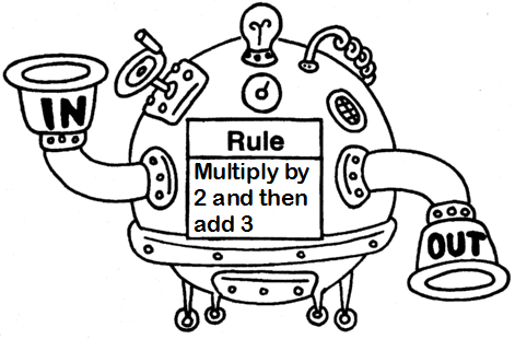
A function \(f: X \rightarrow Y\) from set \(X\) to set \(Y\) is a mapping that associates to each element of \(X\) a uniquely determined element of \(Y\).

• Here we will be interested in the case where \(X\) is a subset of \(\mathbb{R}^n\) and \(Y\) is a subset of \(\mathbb{R}\)

Definition

A single-real-valued multivariate function takes as input \(n\) real numbers and outputs a single real number,

\[ f: \mathbb{R}^{n} \supseteq X \to Y \subseteq \mathbb{R} \]

\[ f: \mathbb{R}^{n} \ni x \mapsto y \in \mathbb{R} \]

Recall that:

• \(X\) is the domain of \(f\).

• \(Y\) is the codomain (target space) of \(f\).

Often we simply write a single-real-valued multivariate functions as

\[ y = f(x_1,x_2,\dots,x_n), \]

where \(x_i\) are the arguments of the function (independent variables) and \(y\) is the function output (dependent variable).

Sometimes vectors \(x \in \mathbb{R}^n\) are written with bold letters, e.g. \(\mathbf{x}=(x_1,x_2,\dots,x_n)\), and multivariate function as \(f(\mathbf{x})=f(x_1,x_2,\dots,x_n)\).

Example

Consider Cobb-Douglas production function \(f: \mathbb{R}^2 \to \mathbb{R}\) given by

\[ f(k, \ell) = k^{\alpha} \ell^{\beta}, \quad \alpha \ge 0, \, \beta \ge 0, \, \alpha + \beta \leqslant 1 \]

• \(k\) input is the amount of capital

• \(\ell\) input is the amount of labor

• the function ouput in \(\mathbb{R}\) is the amount of output produced

Example

Consider the single-real-valued multivariate function \(f(x_1,x_2) = \sqrt{x_1 - 1} + \sqrt{x_2 - 2}\).

• the domain of \(f\) is \(\left\{ (x_1,x_2) \in \mathbb{R}^{2} :\; x_1 \geq 1, x_2 \geq 2 \right\}\).

• the codomain of \(f\) is \(\left\{ y \in \mathbb{R} :\; y \geq 0 \right\}\).

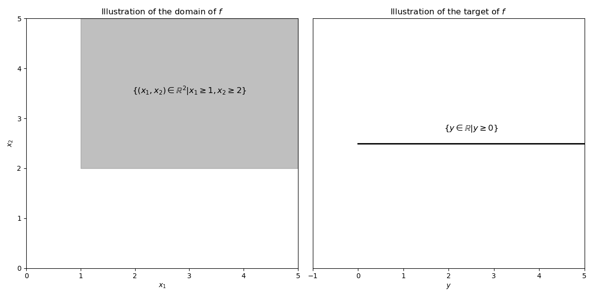
Fig. 41 Illustrations of domain and target space of \(f\).

Graph of two-dimensional functions

Recall that the graph of a function \(f: X \to Y\) is a subset of the Cartesian product \(X \times Y\) given by \(\{(x,y) \in X \times Y: y = f(x)\}\)

For the two-dimensional functions from \(\mathbb{R}^2\) to \(\mathbb{R}\), the graph is a subset of \(\mathbb{R}^3\), and thus we can visualize it is a picture.

The graph is a surface in \(\mathbb{R}^3\), or a height map - surface - ``blanket’’ over the usual Eucledian \(x\)-\(y\) plane

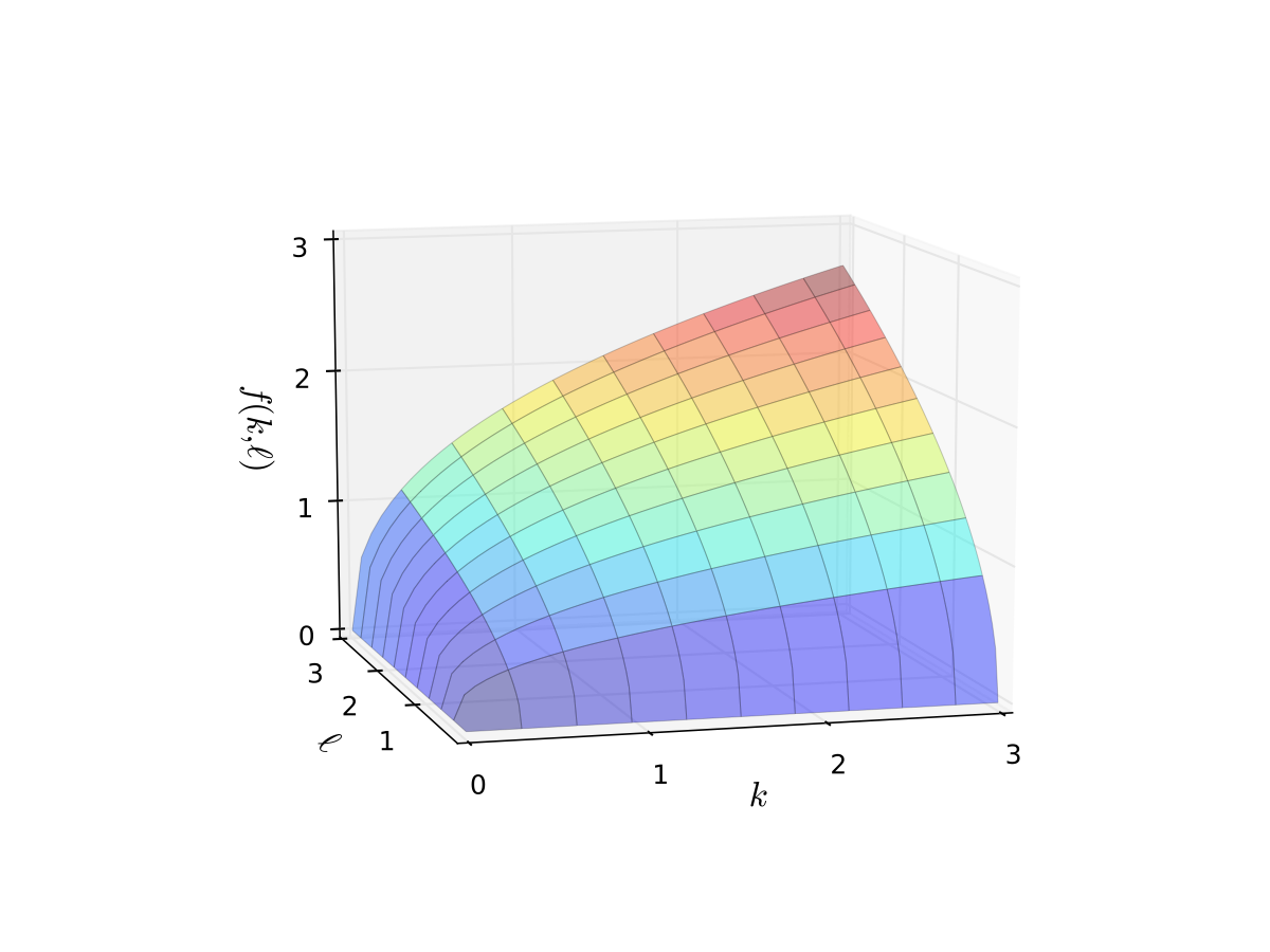
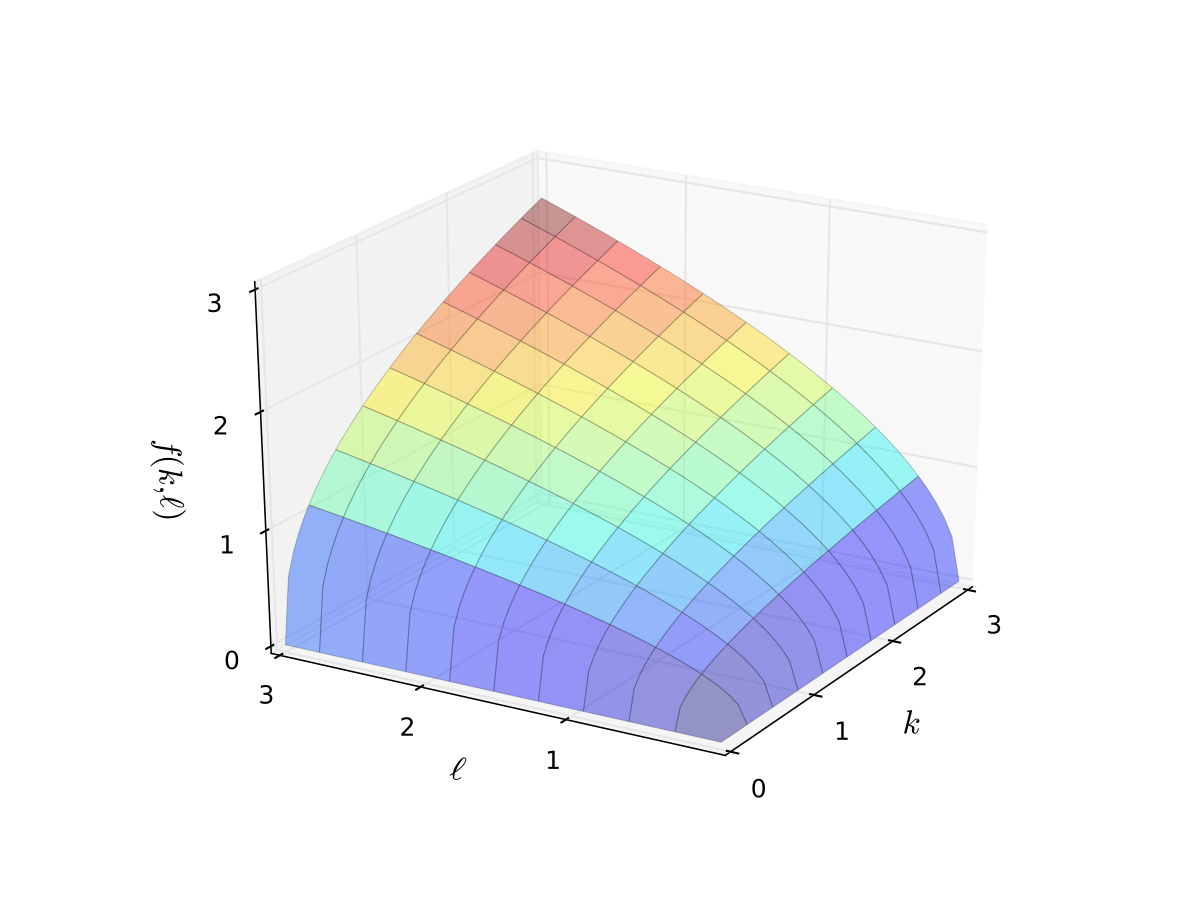
Example

Production function \(f(k, \ell) = k^{\alpha} \ell^{\beta}\) with \(\alpha=0.4\), \(\beta=0.5\)

We can rotate the graph to see it from different angles

Level curves and sets

Definition

A set \(M\) in \(\mathbb{R}^n\) is called a level set of \(f(x_1,x_2,\dots,x_n)\) if the value of \(f\) on every point of \(M\) is some fixed \(c\).

Example

\(x^2 + y^2 = c\) defines a level set of \(f(x,y)=x^2 + y^2\)

Depending on the dimension \(n\) level sets have more specific names:

• for \(n=2\) level sets are called level curves, also referred to as contours or isoquants

• for \(n=3\) level sets are called level surfaces

• for \(n>3\) level sets are called level hypersurfaces

Example

\(x^2 + y^2 - z = c\) is the level surface of \(g(x,y,z)=x^2 + y^2 - z\)

Definition

A curve \(\ell\) in \(\mathbb{R}^2\) is called a level curve of \(y=f(x_1,x_2)\) if the value of \(f\) on every point of \(\ell\) is some fixed \(c\):

\[ \ell_c = \{(x_1,x_2) \in \mathbb{R}^2 : f(x_1,x_2) = c\} \]

Level curves can also be used to visualize bivariate functions, \(f: X \subset \mathbb{R}^2 \rightarrow Y \subset \mathbb{R}\).

Example

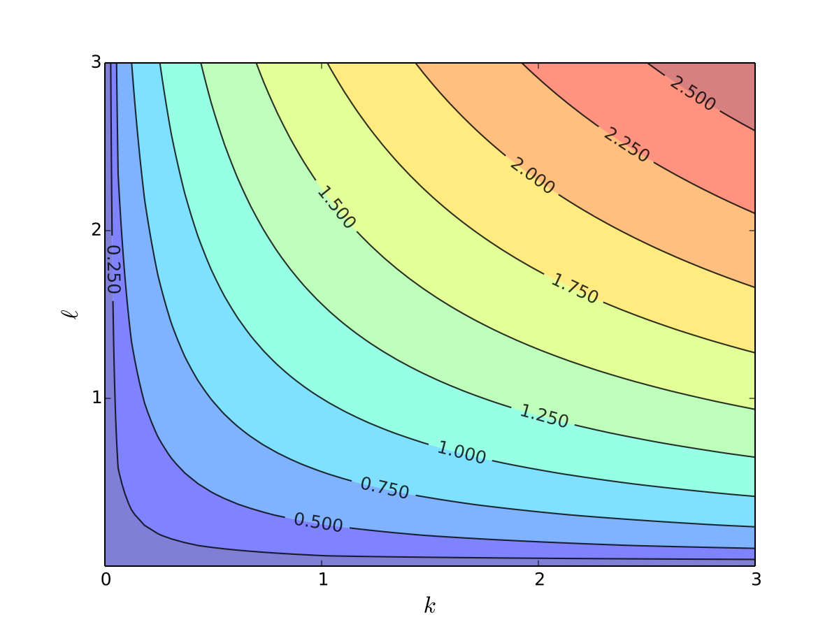
Level curves for the production function \(f(k, \ell) = k^{\alpha} \ell^{\beta}\) with \(\alpha=0.4\), \(\beta=0.5\)

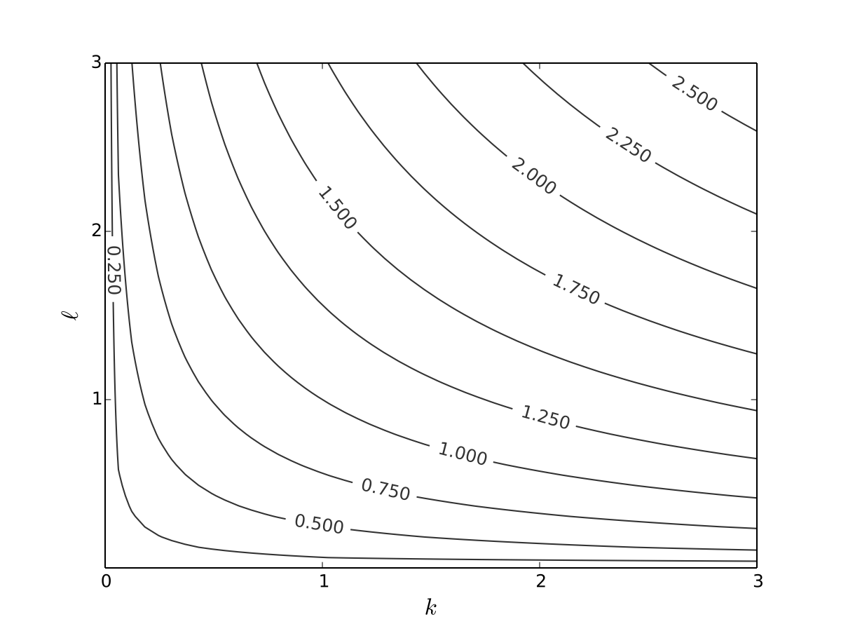
Exercise: Can you see how \(\alpha < \beta\) shows up in the slope of the contours?

A lot of the times adding colors of the hight map together with the contour lines makes for a better visualization

Examples of bivariate functions in economics

In economic analysis we will often use single-real-valued multivariate functions to represent

• production functions

• cost functions

• profit functions

• utility functions

• demand functions

Example

Important single-real-valued bivariate functions used in economic analysis:

• Linear function

\[f(\mathbf{x}) = a_{1} x_{1} + a_{2} x_{2}.\]

• Input-output function

\[f(\mathbf{x}) = \text{min}(a_1 x_1, a_2 x_2).\]

• Cobb-Douglas function

\[f(\mathbf{x}) = k x_{1}^{b_1} x_{2}^{b_2}.\]

• Constant elasticity of substitution (CES) function,

\[f(\mathbf{x}) = k (c_1 x_1^{a} + c_2 x_2^{a})^{b/a}.\]

These functions are straight forward to extent to more than two inputs.

Example: log-utility

Let \(u(x_1,x_2)\) be “utility” gained from \(x_1\) units of good 1 and \(x_2\) units of good 2

We take

\[ u(x_1, x_2) = \alpha \log(x_1) + \beta \log(x_2) \]

where

• \(\alpha\) and \(\beta\) are parameters

• we assume \(\alpha>0, \, \beta > 0\)

• The log functions mean “diminishing returns” in each good

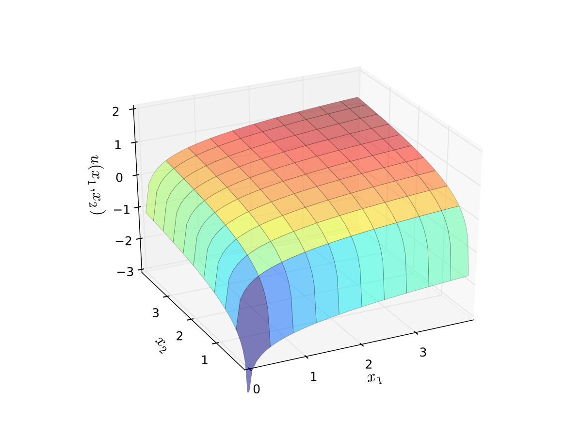
Fig. 42 Log utility with \(\alpha=0.4\), \(\beta=0.5\)

Let’s look at the contour lines

For utility functions, contour lines called indifference curves

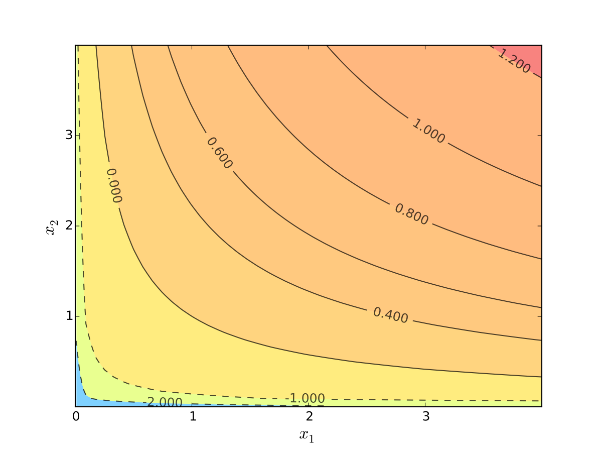
Fig. 43 Indifference curves of log utility with \(\alpha=0.4\), \(\beta=0.5\)

Example: quasi-linear utility

\[ u(x_1, x_2) = x_1 + \log(x_2) \]

• Called quasi-linear because linear in good 1

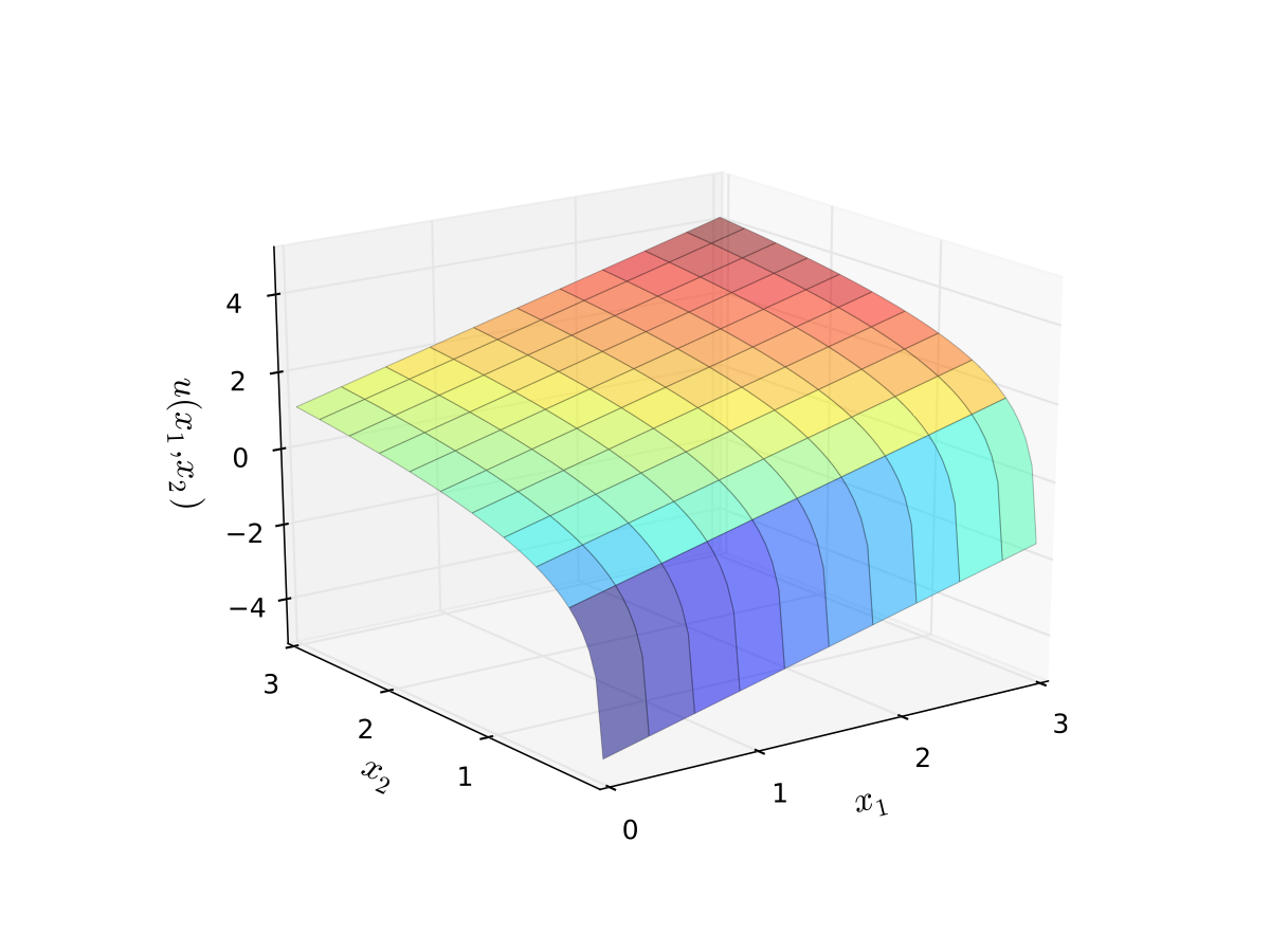
Fig. 44 Quasi-linear utility

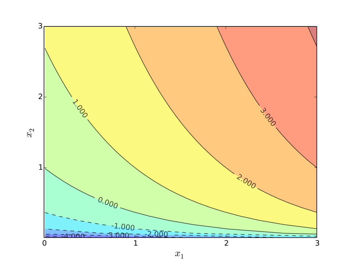
Fig. 45 Indifference curves of quasi-linear utility

Example: quadratic utility

\[ u(x_1, x_2) = - (x_1 - b_1)^2 - (x_2 - b_2)^2 \]

Here

• \(b_1\) is a “satiation” or “bliss” point for \(x_1\)

• \(b_2\) is a “satiation” or “bliss” point for \(x_2\)

Dissatisfaction increases with deviations from the bliss points

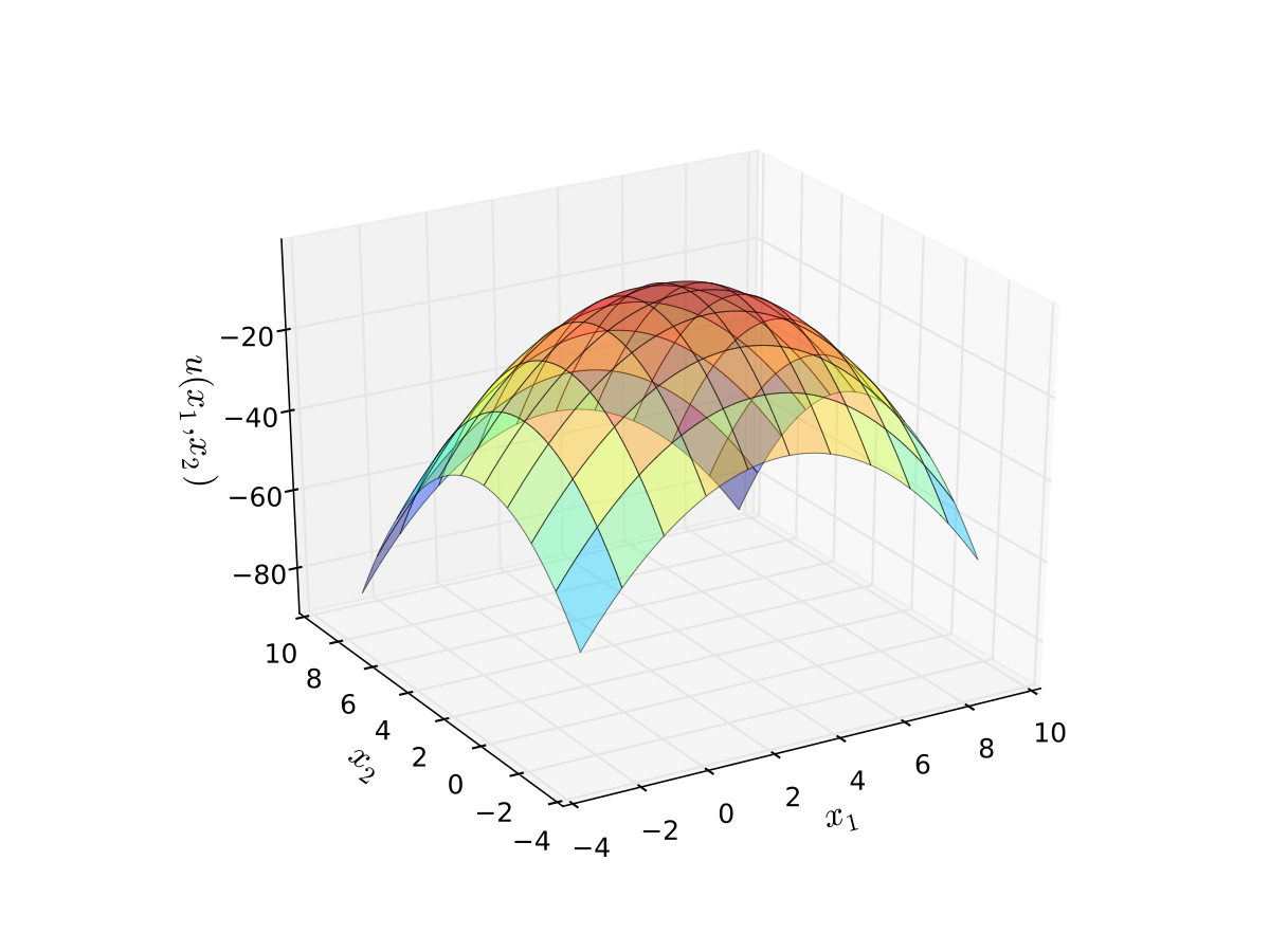
Fig. 46 Quadratic utility with \(b_1 = 3\) and \(b_2 = 2\)

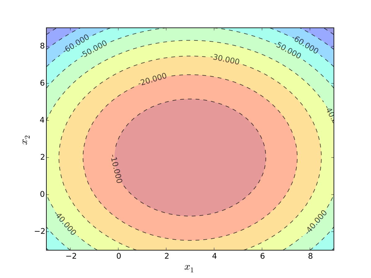
Fig. 47 Indifference curves quadratic utility with \(b_1 = 3\) and \(b_2 = 2\)

Partial derivatives

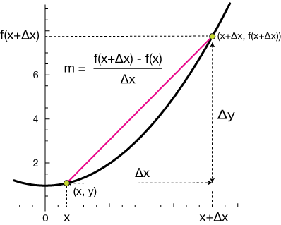
Recall that for univariate functions \(f: \mathbb{R} \to \mathbb{R}\) we defined the derivative at the point \(x\), if it exists, to be the limit of the slope of the secant line as the step size \(\Delta x\) approaches zero

\[ f^{\prime}\left(x\right) =\frac{d f}{d x}(x) =\lim _{\Delta x \rightarrow 0} \frac{f\left(x+\Delta x\right)-f\left(x\right)}{\Delta x} . \]

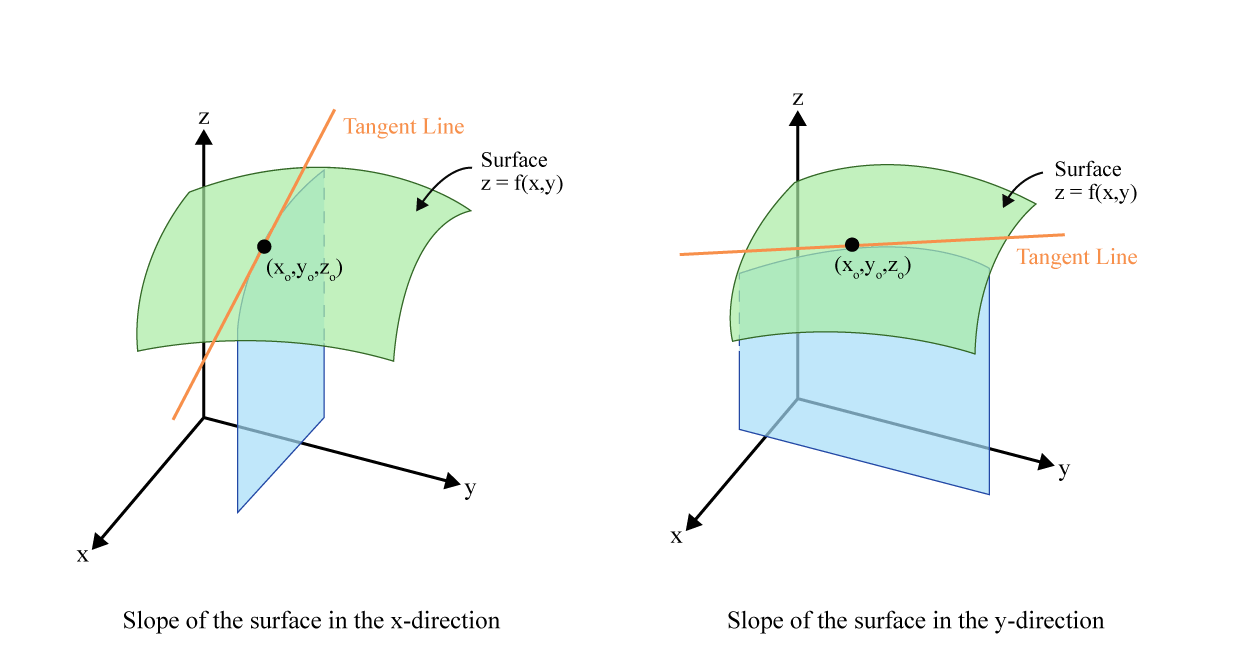
How to differentiate a function of several variables?

Perhaps we should proceed variable by variable, one at a time.

Suppose that we hold the values of \((n-1)\) of function arguments constant and only allow the k’th independent variable to take on different values, \(x_k\).

Let \(\mathbf{x}_{-k}\) denote the \((n-1)\) independent variables we keep fixed

\[ \mathbf{x}_{-k}=\left(x_{1}, x_{2}, \dots, x_{k-1}, x_{k+1}, \dots, x_{n}\right) \]

We can now think about the multivariate function as a univariate function \(f(x_1,\dots,x_n)\) as if it had only \(x_{k}\) as independent variable.

To be precise, we have

\[ g\left(x_{k}\right)=f\left(x_{k}; \mathbf{x}_{-k}\right) . \]

Suppose that the univariate function \(g\left(x_{k}\right)\) is differentiable, so we can write \(g^{\prime}\left(x_{k}\right)=\frac{d g\left(x_{k}\right)}{d x_{k}}\) — it is this derivative that we will call the partial derivative of \(f\) with respect to \(x_{k}\).

Definition

The partial derivative of the single-real-valued multivariate function \(f: \mathbb{R}^n \to \mathbb{R}\) with respect to the variable \(x_{k}\) is defined as

\[ f'_k(\mathbf{x}) = \frac{\partial f\left(\mathbf{x}\right)}{\partial x_{k}} = \lim _{h \rightarrow 0}\left\{\frac{f\left(x_{1}, \dots, x_{k} + h, x_{k+1}, \dots, x_n\right) - f\left(x_{1}, \dots, x_{k}, x_{k+1}, \dots, x_n\right)}{h}\right\} . \]

Note the notation for the partial derivative: short notation \(f'_k(\mathbf{x})\) or in some contexts even dropping the apostrophe \(f_k(\mathbf{x})\), and the full and better notation is \(\frac{\partial f\left(\mathbf{x}\right)}{\partial x_{k}}\), which is different from \(\frac{d f}{d x}(x)\) in the use of new symbol ``\(\partial\)’’.

So, for a function \(f: \mathbb{R}^n \to \mathbb{R}\) we have \(n\) different partial derivatives!

Example

\[f(\mathbf{x}) = a_{1} x_{1} + a_{2} x_{2}.\]

\[ \frac{\partial f(x_1,x_2)}{\partial x_1} = a_{1}, \quad \frac{\partial f(x_1,x_2)}{\partial x_2} = a_{2} \]

Example

\[f(\mathbf{x}) = \text{min}(a_1 x_1, a_2 x_2).\]

\[\begin{split} \frac{\partial f(x_1,x_2)}{\partial x_1} = \begin{cases} a_1 & \text{if } a_1 x_1 < a_2 x_2 \\ 0 & \text{if } a_1 x_1 > a_2 x_2 \\ \end{cases} \qquad \frac{\partial f(x_1,x_2)}{\partial x_2} = \begin{cases} a_2 & \text{if } a_1 x_1 > a_2 x_2 \\ 0 & \text{if } a_1 x_1 < a_2 x_2 \\ \end{cases} \end{split}\]

Exercise: What about the equality case?

Example

\[f(\mathbf{x}) = k (c_1 x_1^{a} + c_2 x_2^{a})^{b/a}.\]

When computing partial derivative we treat the remaining independent variables as constants

\[ \frac{\partial f(x_1,x_2)}{\partial x_1} = kb c_1 (c_1 x_1^{a} + c_2 x_2^{a})^{(b/a)-1} x_1^{a-1} \]

\[ \frac{\partial f(x_1,x_2)}{\partial x_2} = kb c_2 (c_1 x_1^{a} + c_2 x_2^{a})^{(b/a)-1} x_2^{a-1} \]

Note that the partial derivative, \(\frac{\partial f\left(\mathbf{x}\right)}{\partial x_k}\), is a single-real-valued multivariate function itself, as it in general depend on all the independent variables. Like simple derivatives, partial derivatives are computed at a point in the domain of the function in \(\mathbb{R}^n\).

Differentiability of multivariate functions

Definition

A function \(f: \mathbb{R}^n \to \mathbb{R}\) is said to be differentiable at the point \(\mathbf{x}^*\) if there exists all partial derivatives at that point.

Definition

A function \(f: \mathbb{R}^n \to \mathbb{R}\) is said to be continuously differentiable at the point \(\mathbf{x}^*\) if all partial derivatives exist and are continuous in a neighborhood of \(\mathbf{x}^*\).

• All similar to the univariate case

Rules for partial derivatives

Note that when calculating the partial derivative with respect \(x_k\) we treat the remaining independent variables as constants. Hence, we can use the same rules for partial differentiation as for differentiation of univariate functions.

Fact: Rules for partial differentiation

• \(f(\mathbf{x}) = c g(\mathbf{x}) \implies f'_k\left( \mathbf{x} \right) = c g'_k\left( \mathbf{x} \right)\)
  

• \(f(\mathbf{x}) = g(\mathbf{x}) + h(\mathbf{x}) \implies f'_k\left( \mathbf{x} \right) = g'_k\left( \mathbf{x} \right) + h'_k\left( \mathbf{x} \right)\)

• \(f(\mathbf{x}) = g(\mathbf{x})h(\mathbf{x}) \implies f'_k\left( \mathbf{x} \right) = g'_k(\mathbf{x})h(\mathbf{x}) + g(\mathbf{x})h'_k(\mathbf{x})\)

Example

\[ \frac{\partial}{\partial x_1} \left( \lambda e^{x_1} + \lambda \ln(x_2) \right) = \lambda \frac{\partial}{\partial x_1} \left( e^{x_1} + \ln(x_2) \right) = \lambda e^{x_1} \]

\[ \frac{\partial}{\partial x_2} \left( \lambda e^{x_1} + \lambda \ln(x_2) \right) = \lambda \frac{\partial}{\partial x_2} \left( e^{x_1} + \ln(x_2) \right) = \frac{\lambda}{x_2} \]

\[ \frac{\partial}{\partial x} \left( x^2 + xy + y^3 \right) = \frac{\partial}{\partial x} \left( x^2 \right) + \frac{\partial}{\partial x} \left( xy \right) + \frac{\partial}{\partial x} \left( y^3 \right) = 2x + y + 0 = 2x + y \]

\[ \frac{\partial}{\partial x} \left( x^2 y \ln(xy) \right) = y\left[ \frac{\partial}{\partial x} \left( x^2 \right) \ln(xy) + \frac{\partial}{\partial x} \left( \ln(xy) \right) x^2 \right] = y\left[ 2x \ln(xy) + \frac{x^2}{xy}y \right] = 2xy\ln(xy) + xy \]

Differentiation of composite functions

• composition of functions of many variables requires a bit more attention to make sure that the range of the inner function is in the domain of the outer function

• multivariate function also allow for more involved compositions, with the corresponding adjustment of the chain rule

Fact

Consider the function \(f: \mathbb{R}^n \to \mathbb{R}\) and functions \(g_i: \mathbb{R}^m \to \mathbb{R}\) for \(i=1,\dots,n\)

The derivative of the composition \(f\big(g_1(\mathbf{x}),\dots,g_n(\mathbf{x})\big)\) is given by

\[ \frac{\partial f\big(g_1(\mathbf{x}),\dots,g_n(\mathbf{x})\big)}{\partial x_k} = \sum_{i=1}^{n} \frac{\partial f\big(g_1(\mathbf{x}),\dots,g_n(\mathbf{x})\big)}{\partial g_i} \frac{\partial g_i(\mathbf{x})}{\partial x_k} \]

• this rule is a special case of the more general multivariate chain rule

• with multiple variables there are more combinations of the functions in the composition, and therefore more versions of the chain rule

• matrix algebra is used to deal with the more complex cases after forming vectors and matrices of partial derivatives

• we will look more at this in the next lecture

Example

Consider

\[ f(y_1,y_2,y_3) = y_1^2 + y_2^2+ y_3^2 \]

\[\begin{split} \begin{array}{c} g_1(x_1,x_2) = a_1\exp(x_1^2) + b_1\exp(x_2^2) \\ g_2(x_1,x_2) = a_2\exp(x_1^2) + b_2\exp(x_2^2) \\ g_3(x_1,x_2) = a_3\exp(x_1^2) + b_3\exp(x_2^2) \\ \end{array} \end{split}\]

Then the partial derivative of the composite function \(f(g_1,g_2,g_3)\) with respect to \(x_1\) is

\[\begin{split} \begin{array}{c} \frac{\partial f\big(g_1(x_1,x_2),g_2(x_1,x_2),g_3(x_1,x_2)\big)}{\partial x_1} = \\ \sum_{j=1}^{3} \frac{\partial f\big(g_1(x_1,x_2),g_2(x_1,x_2),g_3(x_1,x_2)\big)}{\partial g_j} \frac{\partial g_j(x_1,x_2)}{\partial x_1} = \\ \frac{\partial f(y_1,y_2,y_3)}{\partial y_1} \frac{\partial g_1(x_1,x_2)}{\partial x_1} + \frac{\partial f(y_1,y_2,y_3)}{\partial y_2} \frac{\partial g_2(x_1,x_2)}{\partial x_1} + \frac{\partial f(y_1,y_2,y_3)}{\partial y_3} \frac{\partial g_3(x_1,x_2)}{\partial x_1} = \\ 2 g_1(x_1,x_2) \frac{\partial g_1(x_1,x_2)}{\partial x_1} + 2 g_2(x_1,x_2) \frac{\partial g_2(x_1,x_2)}{\partial x_1} + 2 g_3(x_1,x_2) \frac{\partial g_3(x_1,x_2)}{\partial x_1} = \\ 4a_1 g_1(x_1,x_2) x_1 \exp(x_1^2) + 4a_2 g_2(x_1,x_2) x_1 \exp(x_1^2) + 4a_3 g_3(x_1,x_2) x_1 \exp(x_1^2) = \\ 4 x_1 \exp(x_1^2) \left[ a_1 g_1(x_1,x_2) + a_2 g_2(x_1,x_2) + a_3 g_3(x_1,x_2) \right] \end{array} \end{split}\]

Similarly, the partial derivative of the composite function \(f(g_1,g_2,g_3)\) with respect to \(x_2\) is

\[\begin{split} \begin{array}{c} \frac{\partial f\big(g_1(x_1,x_2),g_2(x_1,x_2),g_3(x_1,x_2)\big)}{\partial x_2} = \\ \sum_{j=1}^{3} \frac{\partial f\big(g_1(x_1,x_2),g_2(x_1,x_2),g_3(x_1,x_2)\big)}{\partial g_j} \frac{\partial g_j(x_1,x_2)}{\partial x_2} = \\ \frac{\partial f(y_1,y_2,y_3)}{\partial y_1} \frac{\partial g_1(x_1,x_2)}{\partial x_2} + \frac{\partial f(y_1,y_2,y_3)}{\partial y_2} \frac{\partial g_2(x_1,x_2)}{\partial x_2} + \frac{\partial f(y_1,y_2,y_3)}{\partial y_3} \frac{\partial g_3(x_1,x_2)}{\partial x_2} = \\ 2 g_1(x_1,x_2) \frac{\partial g_1(x_1,x_2)}{\partial x_2} + 2 g_2(x_1,x_2) \frac{\partial g_2(x_1,x_2)}{\partial x_2} + 2 g_3(x_1,x_2) \frac{\partial g_3(x_1,x_2)}{\partial x_2} = \\ 4b_1 g_1(x_1,x_2) x_2 \exp(x_2^2) + 4b_2 g_2(x_1,x_2) x_2 \exp(x_2^2) + 4b_3 g_3(x_1,x_2) x_2 \exp(x_2^2) = \\ 4 x_2 \exp(x_2^2) \left[ b_1 g_1(x_1,x_2) + b_2 g_2(x_1,x_2) + b_3 g_3(x_1,x_2) \right] \end{array} \end{split}\]

Calculating the growth rate of the production

Let the production of the economy is given by the Cobb-Douglas production function \(y=f(L(t),K(t))\) where the labor and capital inputs are both functions of time.

Using ``dot notation’’, let labor and capital is accumulated at constant growth rates \(g_\bullet\)

\[\begin{split} \begin{array}{c} \dot{L} \equiv \frac{dL}{dt} = g_L L(t) \\ \dot{K} \equiv \frac{dK}{dt} = g_K K(t) \end{array} \end{split}\]

Use chain rule to calculate how production changes over time

\[\begin{split} \begin{array}{rl} \frac{dy}{dt} &= \frac{\partial f(L,K)}{\partial L} \frac{dL}{dt} + \frac{\partial f(L,K)}{\partial K} \frac{dK}{dt} \\ &= \alpha A L^{\alpha-1} K^{\beta} g_L L + \beta A L^{\alpha} K^{\beta-1} g_K K \\ &= \alpha A L^{\alpha} K^{\beta} g_L + \beta A L^{\alpha} K^{\beta} g_K \\ &= (\alpha g_L + \beta g_K) y \end{array} \end{split}\]

Divide both sides with the production, \(y\)

\[ \frac{\dot{y}}{y} = \alpha g_L + \beta g_K. \]

The growth rate of the economy is constant, and is given by dot product of the elasticities and growth rates with respect to each of the production inputs.

Implicit functions

Multivariate functions can be used to represent implicit relationships between variables.

Until now we have been working with explicit functions where the dependet variable, \(y\), is on the left side of the equation and the independet variables, \(x_i\), are on the right side

\[ y = f(x_1,x_2,\dots,x_n). \]

Frequently, we have to work with equations where the dependent variable cannot be separated from the independent variables

\[ G(x_1,x_2,\dots,x_n,y) = c. \]

We say that \(G(x_1,x_2,\dots,x_n,y) = c\) represent a relationship between \(y\) and \(x\) that defines an implicit function \(y\) of \(x\).

Example

Suppose that \(f: \mathbb{R}_{+}^{2} \rightarrow \mathbb{R}_{+}\) is a production function.

\[ Q = f(K,L). \]

The level curve of the production function represent a relationship between the capital (\(K\)) and labor (\(L\)) inputs that keeps the production constant at \(Q_0\)

\[ f(K,L) = Q_0. \]

Given the specified production function we might be able to find an explicit or implicit function for the isoquant curve, \(L=g(K)\).

Thus, the multivariate function \(f(K,L)\) defines an implicit function \(L=g(K)\) with the equation \(f(K,L) = Q_0\).

When dealing with implicit functions we want to know the following two answers:

1. Does \(G(x_1,x_2,\dots,x_n,y) = c\) determine \(y\) as a continuous implicit function of \((x_1,x_2,\dots,x_n)\)?

2. If so, how does changes in \(x\) affect \(y\), in other words what is the derivative of \(y\) with respect to \(x\)?

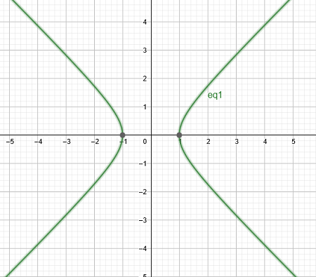
Example

Equation \(x^2-y^2=1\) does not define \(y\) as a function of \(x\)

Now, let’s carry this computation out more generally for the implicit function \(G(x,y)=c\) around the specific point \(x=x^*\), \(y=y^*\), and let’s suppose there exist a function \(y=h(x)\).

Using the chain rule we can differentiate \(G(x,h(x))\)

\[ \frac{d G\big(x, h(x)\big)}{d x} = \frac{\partial G\big(x, h(x)\big)}{\partial x} + \frac{\partial G\big(x, h(x)\big)}{\partial h} \frac{d h(x)}{dx}, \]

Note the difference between the total derivative of \(G(x,h(x))\) with respect to \(x\) as if it was a univariate function of \(x\), and the partial derivative of \(G(x,y)\) with respect to \(x\) as it’s first argument.

Now, differentiating both sides of the equation \(G(x,y)=c\) with respect to \(x\) in the point \((x^*,y^*)\) we get

\[ \frac{\partial G\left(x^*, y^*\right)}{\partial x} + \frac{\partial G\left(x^*, y^*\right)}{\partial y} \frac{d h(x^*)}{dx}=0. \]

from which we can solve for the derivative of the implicit function \(y=h(x)\)

\[ \frac{d h(x^*)}{dx} = -\frac{\tfrac{\partial G\left(x^*, h(x^*)\right)}{\partial x} }{\tfrac{\partial G\left(x^*, h(x^*)\right)}{\partial y}} \]

We see that if the solution \(h(x)\) of \(G(x,y)=c\) exists and is differentiable it is necessary that \(\partial G\left(x_0, y(x_0)\right) /\partial y\) be nonezero

The implicit function theorem stated below implies that this necessary condition is also a sufficient condition.

Fact

Let \(G\left(x, y\right)\) be a \(C^1\) function around the point \((x^*,y^*)\) in \(\mathbb{R}^2\). Suppose \(G(x^*,y^*)=c\) and consider the expression

\[ G(x,y)=c. \]

If \(\partial G\left(x^*, h(x^*)\right) / \partial h \neq 0\), then there exists a \(C^1\) function \(y=h(x)\) defined in neighborhood around the point \(x^*\) such that

• \(G(x,h(x)) = c\) for all \(x\) around \((x^*,y^*)\)

• \(h(x^*)=y^*\)

• the derivative of \(h\) wrt \(x\) at \((x^*,y^*)\) is

\[ h'(x) =-\frac{\tfrac{\partial G\left(x^*, h(x^*)\right)}{\partial x} }{\tfrac{\partial G\left(x^*, h(x^*)\right)}{\partial y}}. \]

The implicit function theorem provides conditions under which a relationship of the form \(G(x,y)=c\) implies that there exists a implicit function \(y=h(x)\) locally.

Example

Consider equation of a unit circle \(x^2 + y^2=1\)

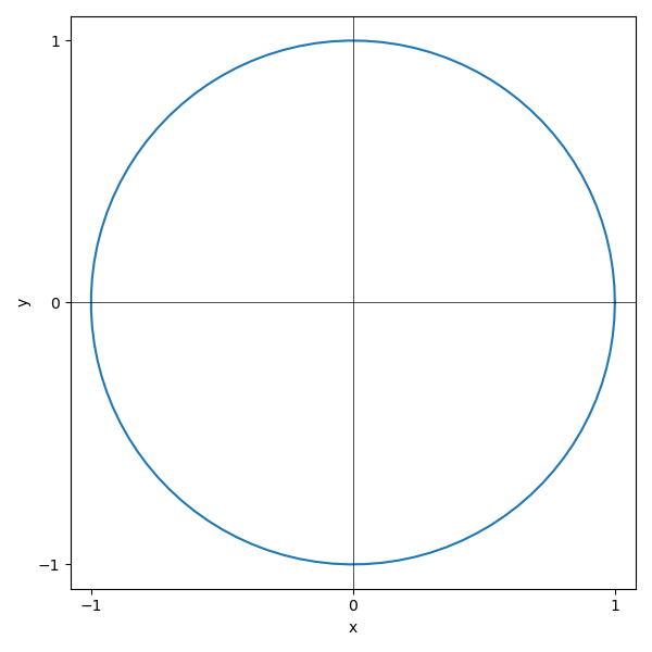
It is clear that in general we can not express \(y\) as a function of \(x\).

Is the implicit function \(y=h(x)\) defined around the point \((0,1)\)?

By implicit function theorem we have

\[ G(x,y) = x^2 + y^2 - 1,\; G'_1(x,y)=\frac{\partial G(x,y)}{\partial x} = 2x,\; G'_2(x,y)=\frac{\partial G(x,y)}{\partial y} = 2y \]

So, at the point \((0,1)\) we have \(G'_1(0,1)=0\) and \(G'_2(0,1)=2 \ne 0\), thus in the neighborhood of the point \((0,1)\) there is a differentiable implicit function

\[ y=h(x); \; \frac{d h(x)}{dx} = -\frac{2x}{2y} = -x/h(x); \; h'(0) = 0 \]

It’s not hard to show that this function is \(h(x) = \sqrt{1-x^2}\) by taking the positive root of corresponding quadratic equation for \(y\).

Simple check also confirms that \(h'(x) = -x/h(x)\):

\[ \frac{d h(x)}{dx} = \frac{d}{dx} \sqrt{1-x^2} = \frac{-2x}{2\sqrt{1-x^2}} = -\frac{x}{h(x)} \]

Is the implicit function \(y=h(x)\) defined around the point \((0,-1)\)?

We have that \(G'_2(0,-1) = -2 \ne 0\) and thus by the implicit function theorem there is a differentiable implicit function \(y=h(x)\) in the neighborhood of the point \((0,-1)\), and \(h'(0) = 0\). It’s not hard to show that this function is \(h(x) = -\sqrt{1-x^2}\), and verify that again \(h'(x) = -x/h(x)\).

Is the implicit function \(y=h(x)\) defined around the point \((1,0)\)?

We have that \(G'_2(1,0) = 0\) and thus by the implicit function theorem the implicit function \(y(x)\) is not defined at this point. Intuitively, because the unit circle is ``vertical’’ at this point, the slope of the tangent line is infinite, and thus there is no local mapping at this point which is a function.

Example

Consider the polynomial equation

\[ y^5 + y^3 + y + x = 0. \]

\(x\) can be expressed as an explicit function of \(y\)

\[ x(y) = - y^5 - y^3 - y. \]

However, polynomials of order \(k \geq 5\) has no explicit solution. Hence, there exist no explicit function \(y\) of \(x\). Instead, the polynomial equation defines an implicit function for \(y\) of \(x\).

Suppose we could find a function \(y=y(x)\) which solves this equation for any \(x\)

\[ y(x)^5 + y(x)^3 + y(x) + x = 0. \]

Use the chain rule to find \(y'(x)\)

\[\begin{split} 5 y(x)^4 y'(x) + 3 y(x)^2 y'(x) + y'(x) + 1 = 0 \\ \Leftrightarrow y'(x) =-\frac{1}{5 y(x)^4 + 3 y(x)^2 + 1} \end{split}\]

The point \(x=-3\), \(y=1\) solves the polynomial equation, and

\[ y'(3)=-\tfrac{1}{5 + 3 + 1} = -\tfrac{1}{8} \]

We conclude that there exists an implicit function \(y=y(x)\) in the neighborhood around (-3,1) that solves polynomial equation and it is differentiable.

Example

Consider the cubic implicit function

\[ x^2 - 3xy + y^3 = 7 \]

around the point \(x=4\), \(y=3\)

\[\begin{split} 4^2 - 3xy + y^3 &= 7 \\ 16 - 36 + 27 &= 7 \\ 7 &= 7 \end{split}\]

Suppose we could find a function \(y=y(x)\) which solves this equation for any \(x\)

\[ x^2 - 3xy(x) + y(x)^3 = 7 \]

use the chain rule to find \(y'(x)\)

\[\begin{split} 2x- 3y(x) - 3xy'(x) + 3y(x)^2 y'(x) = 0 \\ \Leftrightarrow y'(x) =-\frac{2x - 3y}{3y^2 - 3x} \end{split}\]

Alternatively, we could have used total differentiation

\[\begin{split} (2x - 3y)dx + (-3x + 3y^2)dy=0 \\ \Leftrightarrow y'(x)=\frac{dy}{dx} =-\frac{2x - 3y}{3y^2 - 3x} \end{split}\]

at \(x=4\), \(y=3\), we find

\[ y'(x)=-\frac{8-9}{27 - 12}=\frac{1}{15} \]

We conclude that there is a function \(y(x)\) that solve the implicit function around \(x=4\), \(y=3\) and it is differentiable.

Multidimensional implicit function theorem

The implicit function theoriem can be extended to \(G(x_1,x_2,\dots,x_n,y)=c\).

Fact (Implicit function theorem II)

Let \(\mathbf{x}=(x_1,x_2,\dots,x_n)\) and \(G\left(\mathbf{x}, y\right)\) be a \(C^1\) function around the point \((\mathbf{x}^*,y^*)\) in \(\mathbb{R}^{n+1}\). Suppose \(G(\mathbf{x}^*,y^*)=c\) and consider the expression

\[ G(\mathbf{x},y)=c. \]

If \(\partial G\left(\mathbf{x}^*, y(\mathbf{x}^*)\right) / \partial y \neq 0\), then there exists a \(C^1\) function \(y=y(\mathbf{x})\) defined in the neighborhood around the point \(\mathbf{x}^*\) such that

• \(G(\mathbf{x},y(\mathbf{x})) = c\) for all \(\mathbf{x}\) around \((\mathbf{x}^*,y^*)\)

• \(y(\mathbf{x}^*)=y^*\)

• for each \(i\) the derivative of \(y\) wrt \(x_i\) is

\[ \frac{\partial y(\mathbf{x}^*)}{\partial x_i} = -\frac{\tfrac{\partial G\left(\mathbf{x}^*,y^*\right)}{\partial x_i} }{\tfrac{\partial G\left(\mathbf{x}^*,y^*\right)}{\partial y}}. \]

Example: \(G(x,y,z)=c\)

Consider the relationship

\[ - 3 x^2 y + y z - 4 x z = 7. \]

We will show that near \((-1,1,2)\) we can write \(y=y(x,z)\) and we will find the partial \(\partial y / \partial x\) to that point

\[ - 3 \cdot (-1)^2 \cdot 1 + 1 \cdot 2 - 4 \cdot (-1) \cdot 2 = - 3 + 2 + 8 = 7 \]

Find the partial derivatives of \(G\) with respect to \(y\) and \(x\)

\[\begin{split} \begin{array}{c} \frac{\partial G}{\partial x} &= -6xy - 4z. \\ \frac{\partial G}{\partial y} &= -3x^2 + z. \end{array} \end{split}\]

The partial derivative is given by the implicit function theorem as

\[ \frac{\partial y}{\partial x} = -\frac{\tfrac{\partial G}{\partial x} }{\tfrac{\partial G}{\partial y}} = -\frac{-6xy - 4z}{-3x^2 + z} \]

We conclude that there exists a \(C^1\) function \(y=y(x,z)\) in the neighborhood around the point (-1,1,2).

Economic examples and applications

Marginal products of production inputs

Suppose a firm’s production is described by a Cobb-Douglas production function, where labor (L) and capital (K) are the inputs:

\[ Q = f(L, K)=A L^{\alpha} K^{\beta} . \]

The marginal product of labour is simply the partial derivative with respect to labor. Thus we have

\[\begin{split} \begin{aligned} M P_{L}(L, K) & =\frac{\partial f(L, K)}{\partial L} \\ & =\frac{\partial\left(A L^{\alpha} K^{\beta}\right)}{\partial L} \\ & =\alpha A L^{\alpha-1} K^{\beta} \end{aligned} \end{split}\]

The marginal product of capital is simply the first-order derivative with respect to capital. Thus we have

\[\begin{split} \begin{aligned} M P_{K}(L, K) & =\frac{\partial f(L, K)}{\partial K} \\ & =\frac{\partial\left(A L^{\alpha} K^{\beta}\right)}{\partial K} \\ & =\beta A L^{\alpha} K^{\beta-1} \end{aligned} \end{split}\]

The slope of an isoquant curve

Suppose that \(f: \mathbb{R}_{+}^{2} \rightarrow \mathbb{R}_{+}\) is a production function.

\[ Q = f(K,L). \]

The level curve of the production function represent a relationship between the capital (K) and labor (L) inputs that keeps the production constant at \(c\)

\[ f(K,L) = c. \]

Given the specified production function we might be able to find an explicit or implicit function for the isoquant curve, \(L=L(K)\). In both cases we can use the implicit function theorem to calculate the slope of the isoquant curve.

\[\begin{split} \frac{\partial f(K,L)}{\partial K} + \frac{\partial f(K,L)}{\partial L} \frac{\partial L(K)}{\partial K} = 0 \\ \Leftrightarrow \frac{\partial L(K)}{\partial K} = -\frac{\tfrac{\partial f(K,L)}{\partial K}}{\tfrac{\partial f(K,L)}{\partial L}} \end{split}\]

The (negation of) slope of the isoquant curve is referred to as the marginal rate of technical substitution

\[ \text{MRTS}_{LK} = \frac{\tfrac{\partial f(K,L)}{\partial K}}{\tfrac{\partial f(K,L)}{\partial L}}. \]

It measures how much of one input would be needed to compensate for a one-unit loss of the other while keeping the production at the same level.

Marginal rate of (technical) substitution between input \(x_i\) and \(x_j\) of a multivariate function is similarly given by partial derivatives as

\[ \text{MRTS}_{x_i,x_j} = \frac{\tfrac{\partial f(x_1,x_2,\dots,x_n)}{\partial x_j}}{\tfrac{\partial f(x_1,x_2,\dots,x_n)}{\partial x_i}}. \]

MRTS with three inputs

Consider the level surface of the Cobb-Douglas function of three inputs (capital, labor, and land)

\[ A C^{\alpha} L^{\beta} T^{\delta} = c \]

Calculate the marginal rate of substitution between capital and labor

\[\begin{split} \alpha A C^{\alpha-1} L^{\beta} T^{\delta} \frac{\partial C(L,T)}{\partial L} + \beta A C^{\alpha} L^{\beta-1} T^{\delta} = 0 \\ \Leftrightarrow \frac{\partial C(L,T)}{\partial L} = -\frac{\beta A C^{\alpha} L^{\beta-1} T^{\delta}}{\alpha A C^{\alpha-1} L^{\beta} T^{\delta}} = \frac{\beta}{\alpha} \frac{C}{L} \end{split}\]

Calculate the marginal rate of substitution between capital and land

\[\begin{split} \alpha A C^{\alpha-1} L^{\beta} T^{\delta} \frac{\partial C(L,T)}{\partial T} + \delta A C^{\alpha} L^{\beta} T^{\delta-1} = 0 \\ \Leftrightarrow \frac{\partial C(L,T)}{\partial L} = -\frac{\delta A C^{\alpha} L^{\beta} T^{\delta-1}}{\alpha A C^{\alpha-1} L^{\beta} T^{\delta}} = \frac{\delta}{\alpha} \frac{C}{T} \end{split}\]

Calculate the marginal rate of substitution between labor and land

\[\begin{split} \beta A C^{\alpha} L^{\beta-1} T^{\delta}\frac{\partial L(C,T)}{\partial T} + \delta A C^{\alpha} L^{\beta} T^{\delta-1} = 0 \\ \Leftrightarrow \frac{\partial L(C,T)}{\partial T} = -\frac{\delta A C^{\alpha} L^{\beta} T^{\delta-1}}{\beta A C^{\alpha} L^{\beta-1} T^{\delta}} = \frac{\delta}{\beta} \frac{L}{T} \end{split}\]

Homogeneous functions

Homogeneous functions are functions that exhibit a certain scaling property. They are often used in economics to model production functions, utility functions, and other relationships where inputs can be scaled up or down.

Definition

Consider a function \(f: S \to \mathbb{R}\), where \(S \subseteq \mathbb{R}^{n}\), and let \(\lambda>0\) be a positive real number.

The function \(f\left(x_{1}, x_{2}, \cdots, x_{n}\right)\) is said to be homogeneous of degree \(r\) if

\[ f\left(\lambda x_{1}, \lambda x_{2}, \cdots, \lambda x_{n}\right)=\lambda^{r} f\left(x_{1}, x_{2}, \cdots, x_{n}\right) \]

for all \(\left(x_{1}, x_{2}, \cdots, x_{n}\right) \in S\) and all \(\lambda>0\).

Example

The function

\[ 3x^5 y + 2x^2 y^4 - 3 x^3 y^3, \]

is homogenous of degree 6

\[\begin{split} \begin{array}{l} 3(\lambda x)^5 (\lambda y) + 2(\lambda x)^2 (\lambda y)^4 - 3 (\lambda x)^3 (\lambda y)^3 = \\ 3\lambda^5 x^5 \lambda y + 2\lambda^2 x^2 \lambda^4 y^4 - 3 \lambda^3 x^3 \lambda^3 y^3 = \\ 3\lambda^6 x^5 y + 2\lambda^6 x^2 y^4 - 3 \lambda^6 x^3 y^3 = \\ \lambda^6 \left(3 x^5 y + 2 x^2 y^4 - 3 x^3 y^3 \right). \end{array} \end{split}\]

In contrast, the function

\[ 3x^{3/4} y^{1/4} + 6x + 4, \]

is not homogenous

\[ 3(\lambda x)^{3/4} (\lambda y)^{1/4} + 6(\lambda x) + 4 = 3 \lambda x^{3/4} y^{1/4} + 6\lambda x + 4. \]

Fact

Let \(z=f(x)\) be a \(C^1\) function that is homogenous of degree \(r\).

Then its first order partial derivatives are homogenous of degree \(r-1\).

Proof

By definition of homogenous functions we have

\[ f(\lambda x_1, \lambda x_2, \dots, \lambda x_n) = \lambda^r f(x_1,x_2,\dots,x_n). \]

Differentiate both side with respect ot \(x_i\) using chain rule, and divide by \(\lambda\):

\[ \frac{\partial f(\lambda x_1, \lambda x_2, \dots, \lambda x_n)}{\partial x_i} \lambda = \lambda^r \frac{\partial f(x_1,x_2,\dots,x_n)}{\partial x_i} \implies \]

\[ \frac{\partial f(\lambda x_1, \lambda x_2, \dots, \lambda x_n)}{\partial x_i} = \lambda^{r-1} \frac{\partial f(x_1,x_2,\dots,x_n)}{\partial x_i}. \]

Thus, \(\frac{\partial f(\lambda x_1, \lambda x_2, \dots, \lambda x_n)}{\partial x_i}\) is homogenous of degree \(r-1\).

\(\blacksquare\)

Fact

Let \(q=f(x)\) be a \(C^1\) homogenous function on \(\mathbb{R}^n_+\). The tangent planes to the level sets of \(f\) have constant slope along each ray from the origin.

Proof

Idea of the proof:

Consider the homogenous production function on \(\mathbb{R}^2_+\). We want to show that the MRTS is constant along rays from the origin. Let \((\lambda L_0,\lambda K_0)=(L_1, K_1)\). The MRTS between input \(L\) and \(K\) at \((L_1, K_1)\) equals

\[\begin{split} \begin{array}{c} \frac{f_{K}(L_1, K_1)}{f_{L}(L_1, K_1)} &= \frac{f_{K}(\lambda L_0,\lambda K_0)}{f_{L}(\lambda L_0,\lambda K_0)} \\ &= \frac{\lambda^{r-1} f_{K}( L_0, K_0)}{\lambda^{r-1} f_{L}( L_0, K_0)} \\ &= \frac{f_{K}(L_0, K_0)}{f_{L}( L_0, K_0)} \end{array} \end{split}\]

\(\blacksquare\)

Fact (Euler’s theorem)

Suppose that the function \(f\left(x_{1}, x_{2}, \cdots, x_{n}\right)\) is homogeneous of degree \(r\). In this case we have

\[ \sum_{i=1}^{n} x_{i}\frac{\partial f}{\partial x_{i}}\left(\mathbf{x} \right)=r f\left(\mathbf{x}\right). \]

Proof

By the definition of a homogenous function of degree \(r\)

\[ f(\lambda \mathbf{x}) = \lambda^{r} f(\mathbf{x}). \]

Differentiate both sides wrt \(\lambda\) using the chain rule

\[ \sum_{i=1}^{n} x_{i}\frac{\partial f \left(\lambda \mathbf{x} \right)}{\partial x_{i}} = r \lambda^{r-1} f(\mathbf{x}). \]

Evaluating this for \(\lambda=1\) gives the result

\(\blacksquare\)

Returns to scale

Suppose that an \(n\) input and one output production technology can be represented by a homogenous production function of the form

\[ Q=f\left(L_{1}, L_{2}, \cdots, L_{n}\right) . \]

The production technology is said to display:

• constant returns to scale: \(f\left(\lambda L_{1}, \lambda L_{2}, \cdots, \lambda L_{n}\right)=\lambda Q\).

• decreasing returns to scale: \(f\left(\lambda L_{1}, \lambda L_{2}, \cdots, \lambda L_{n}\right)<\lambda Q\).

• increasing returns to scale: \(f\left(\lambda L_{1}, \lambda L_{2}, \cdots, \lambda L_{n}\right)>\lambda Q\).

Thus, production technology that is characterized by a homogenous production function of degree 1 displays has constant returns to scale.

Return to scale in Cobb-Douglas production functions

Suppose that an two input and one output production technology can be represented by a production function of the form

\[ Q=f(L, K)=A L^{\alpha} K^{\beta} . \]

This type of production function is known as a Cobb-Douglas production function.

Suppose that \(\lambda>0\). Note that

\[\begin{split} \begin{aligned} f(\lambda L, \lambda K) & =A(\lambda L)^{\alpha}(\lambda K)^{\beta} \\ & =A \lambda^{\alpha} L^{\alpha} \lambda^{\beta} K^{\beta} \\ & =\lambda^{\alpha+\beta} A L^{\alpha} K^{\beta} \\ & =\lambda^{\alpha+\beta} f(L, K) \end{aligned} \end{split}\]

Thus we know that the Cobb-Douglas production function is homogeneous of degree \((\alpha+\beta)\).

• If \((\alpha+\beta)<1\), then the Cobb-Douglas production function displays decreasing returns to scale;

• If \((\alpha+\beta)=1\), then the Cobb-Douglas production function displays constant returns to scale; and

• If \((\alpha+\beta)>1\), then the Cobb-Douglas production function displays increasing returns to scale.

Homothetic functions

Definition

A function \(v: S \rightarrow \mathbb{R}\), \(S \subset \mathbb{R}_{+}^n\), is called homothetic if it can be represented as a composition of a strictly increasing function, \(g: \mathbb{R} \rightarrow \mathbb{R}\), and a homogenous function, \(u: S \rightarrow \mathbb{R}\).

\[ v(x) = g\big(u(\mathbf{x})\big) \]

for all \(\mathbf{x}\) in \(S\).

Example: \(G(x,y,z)=c\)

The two functions

\[\begin{split} v_1(x,y)=x^3y^3 + xy \\ v_2(x,y)=xy + 1, \end{split}\]

are homothetic functions with \(u(x,y)=xy\) and the monotonic transformations

\[\begin{split} g_1(x,y) = z^3 + z \\ g_2(x,y) = z + 1, \end{split}\]

respectively.

Fact

Let \(u: \mathbb{R}_{+}^n \rightarrow \mathbb{R}\) be a strictly increasing function. Then, \(u\) is a homothetic if and only if for all \(\mathbf{x}\) and \(\mathbf{y}\) in \(\mathbb{R}^n_+\),

\[ u(\mathbf{x}) \geq u(\mathbf{y}) \Leftrightarrow u(\alpha \mathbf{x}) \geq u(\alpha \mathbf{y}) \text{ for all } \alpha > 0. \]

Fact

Let \(u\) be a \(C^1\) function on \(\mathbb{R}^n_+\). If \(u\) is homothetic then the slopes of the tangent planes of the level sets of \(u\) are constant along each ray from the origin.

Elasticity of substitution

Another economic consept that can be setup nice and cleanly given our recent material.

Recall that elasticity of any one quantity \(y\) with respect to another quantity \(x\), where \(y=f(x)\), is given by

\[ \epsilon^{f}_{x}(x)= \lim_{r \to 0} \frac{\frac{f\big(x(1+r)\big)}{f(x)}-1}{r} = \frac{d f(x)}{d x}\left/\frac{f(x)}{x}\right. = \frac{x}{f(x)} \frac{d f(x)}{d x} = \frac{d \ln f(x)}{d \ln x} \]

Now consider a level curve of a bivariate function \(f(K,L)\) representing either a production function or a utility function.

As shown in the examples above, if we are interested in how the two factors/products can be substituted for each other while maintaining the same level of output/utility, we can use the implicit function theorem to find the slope of the level curve.

\[ \text{MRS}_{LK} = -\frac{\tfrac{\partial f(K,L)}{\partial K}}{\tfrac{\partial f(K,L)}{\partial L}}. \]

Elasticity of substitution measures the percentage change in the ratio of two inputs/products corresponding to a relative change in the marginal rate of substitution (MRS) between them.

Denote \(\tau = L/K\) a new variable that measures the ratio of the two arguments in \(f\), i.e. the ratio of two factors in the production function or two goods in a utility function.

Elasticity of substitution between two inputs \(K\) and \(L\) is defined as the elasticity of \(\tau\) with respect to \(\text{MRS}_{LK}\):

\[ \epsilon_{MRS}^{\tau} = \frac{d \ln \tau}{d \ln MRS(\tau)} \]

This coefficient measures the percentage change in the ratio of two inputs as the marginal rate of (technical) substitution (MRS or MRTS) changes.

Example

Consider the Cobb-Douglas production function \(f(L, K)=A L^{\alpha} K^{\beta}\) with constant returns to scale \(\alpha+\beta=1\) and \(A=1\).

\[ \text{MRTS}_{LK} = \frac{\tfrac{\partial f(K,L)}{\partial K}}{\tfrac{\partial f(K,L)}{\partial L}} = \frac{A L^\alpha \beta K^{\beta-1}}{A \alpha L^{\alpha-1} K^\beta} = \tfrac{\beta}{\alpha}\tfrac{K}{L} \]

\[ \ln \text{MRTS}_{LK} = \ln \tfrac{\beta}{\alpha} + \ln \tfrac{K}{L} \implies \ln \tfrac{K}{L} = \ln \text{MRTS}_{LK} - \ln \tfrac{\beta}{\alpha} \]

\[ \epsilon_{\text{MRTS}}^{\tfrac{K}{L}} = \frac{d \ln \tfrac{K}{L}}{d \ln \text{MRTS}_{LK}} = \frac{d}{d \ln \text{MRTS}_{LK}} \left( \ln \text{MRTS}_{LK} - \ln \tfrac{\beta}{\alpha} \right) = 1 \]

Example

Consider the CES utility function \(f(\mathbf{x}) = k (c_1 x^{a} + c_2 y^{a})^{b/a}\)

\[ \text{MRS}_{yx} = \frac{\tfrac{\partial f(x,y)}{\partial x}}{\tfrac{\partial f(x,y)}{\partial y}} = \frac{k\tfrac{b}{a}(c_1 x^{a} + c_2 y^{a})^{(b/a)-1} c_1 a x^{a-1}}{k\tfrac{b}{a}(c_1 x^{a} + c_2 y^{a})^{(b/a)-1}c_2 a y^{a-1}} = \frac{c_1}{c_2}\left(\frac{x}{y}\right)^{a-1} \]

\[ \ln\text{MRS}_{yx} = \ln \tfrac{c_1}{c_2} + (a-1) \ln \tfrac{x}{y} \]

\[ \ln \tfrac{y}{x} = - \ln \tfrac{x}{y} = \frac{1}{a-1} \ln \tfrac{c_1}{c_2} -\frac{1}{a-1} \ln\text{MRS}_{yx} \]

\[ \epsilon_{\text{MRS}_{yx}}^{\tfrac{y}{x}} = \frac{d \ln \tfrac{x}{y}}{d \ln \text{MRS}_{yx}} = \frac{1}{1-a} \]

The name stands: CES utility function has constant elasticity of substitution defined by a single parameter \(a\).