Announcements & Reminders
📊 Results of the first online test
Average grade is 87.02 🎉
Next test (April 3) will be harder
There were some questions about this test: will reply individually
If there are issues with questions, they will be resolved and test regraded (this is how your grade may change)
🎥 The remainder of today’s lecture will be recorded
Please watch before the tutorials!
📖 Sequences and convergence#
⏱ | words
References and additional materials
Norm and distance#
First, we have to understand how to measure distance between points in \(\mathbb{R}^n = \times_{i \in \{1,2,··· ,n\}} \mathbb{R} = \mathbb{R} \times \mathbb{R} \times \dots \times \mathbb{R}\)
Definition
The Euclidean norm of \(x \in \mathbb{R}^N\) is defined as
Interpretation:
\(\| x \|\) represents the length of \(x\)
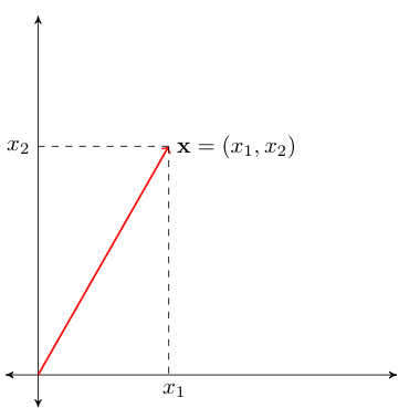
Fig. 21 Length of red line \(= \sqrt{x_1^2 + x_2^2} =: \|x\|\)#
\(\| x - y \|\) represents distance between \(x\) and \(y\)
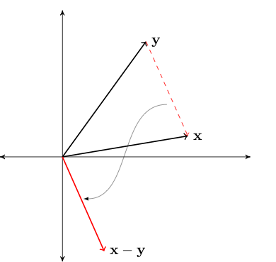
Fig. 22 Length of red line \(= \|x - y\|\)#
Fact
For any \(\alpha \in \mathbb{R}\) and any \(x, y \in \mathbb{R}^N\), the following statements are true:
\(\| x \| \geq 0\) and \(\| x \| = 0\) if and only if \(x = 0\)
\(\| \alpha x \| = |\alpha| \| x \|\)
Triangle inequality
\(\| x + y \| \leqslant \| x \| + \| y \|\)
Proof
For example, let’s show that \(\| x \| = 0 \iff x = 0\)
First let’s assume that \(\| x \| = 0\) and show \(x = 0\)
Since \(\| x \| = 0\) we have \(\| x \|^2 = 0\) and hence \(\sum_{n=1}^N x^2_n = 0\)
That is \(x_n = 0\) for all \(n\), or, equivalently, \(x = 0\)
Next let’s assume that \(x = 0\) and show \(\| x \| = 0\)
This is immediate from the definition of the norm
In fact, any function can be used as a norm, provided that the listed properties are satisfied
Example
More general distance function based on \(\|\cdot\|_\rho\) norm in \(\mathbb{R}^2\).
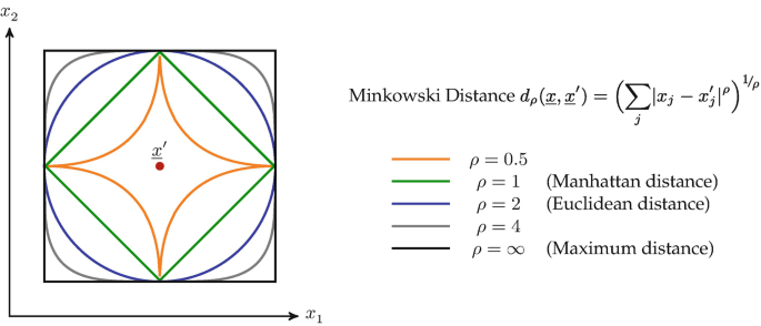
Fig. 23 Circle drawn with different norms#
Absolute value as Euclidean norm in \(\mathbb{R}\)#
Naturally, in \(\mathbb{R}\) Euclidean norm simplifies to
Show code cell source
import numpy as np
import matplotlib.pyplot as plt

def subplots():
    "Custom subplots with axes throught the origin"
    fig, ax = plt.subplots()

    # Set the axes through the origin
    for spine in ['left', 'bottom']:
        ax.spines[spine].set_position('zero')
    for spine in ['right', 'top']:
        ax.spines[spine].set_color('none')

    ax.grid()
    return fig, ax

fig, ax = subplots()

ax.set_ylim(-3, 3)
ax.set_yticks((-3, -2, -1, 1, 2, 3))
x = np.linspace(-3, 3, 100)
ax.plot(x, np.abs(x), 'g-', lw=2, alpha=0.7, label=r'$f(x) = |x|$')
ax.plot(x, x, 'k--', lw=2, alpha=0.7, label=r'$f(x) = x$')
ax.legend(loc='lower right')

plt.show()
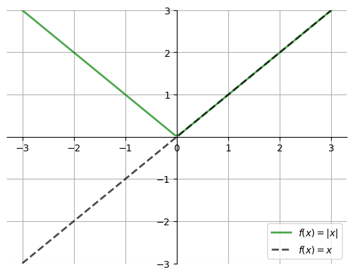
Therefore we can think of norm as a generalization of the absolute value to \(\mathbb{R}\)
Neighborhood of a point#
Fact
For any function \(h(x):\mathbb{R} \to \mathbb{R}\) an inequality of the form
is equivalent to the double inequality
Example
This is equivalent to
Solving the first inequality we have \(x<5\) and solving the second we have \(x>1\). Therefore the solution is \((1,5)\).
Definition
The \(\epsilon\)-neighborhood of a point \(x \in \mathbb{R}\) is the set
\(\epsilon\)-Neighborhood of a point \(x \in \mathbb{R}\) are all the points that are closer to \(x\) than \(\epsilon\).
Sequences#
Definition
A sequence from a set \(X \subset \mathbb{R}\) is a function of the form \(f: \mathbb{N} \rightarrow X\).
It is often denoted by \(\{ x_n \}^\infty_{n=1}\) or \(\{ x_n \}_{n \in \mathbb{N}}\) or \(\{ x_1, x_2, \dots , x_n, \dots \}\), where \(x_n \in X\) for all \(n \in \mathbb{N}\).
In effect, it is indexing of the elements of \(X\) by the natural numbers.
Note that this definition of a sequence does not explicitly allow for finite sequences, but we can think about a finite sequence as being a truncated sequence, where we throw away all terms for which \(n > N\) for some \(N \in \mathbb{N}\). Such a sequence would be written as \(\{ x_n \} ^{N}_{n=1}\) or \(\{ x_1, x_2, \dots , x_{N} \}\).
Example
\(\{x_n\} = \{2, 4, 6, \ldots \}\)
\(\{x_n\} = \{1, 1/2, 1/4, \ldots \}\)
\(\{x_n\} = \{1, -1, 1, -1, \ldots \}\)
\(\{x_n\} = \{0, 0, 0, \ldots \}\)
Convergence and limit#
Let \(a \in \mathbb{R}\) and let \(\{x_n\}\) be a sequence
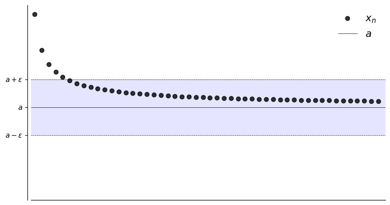
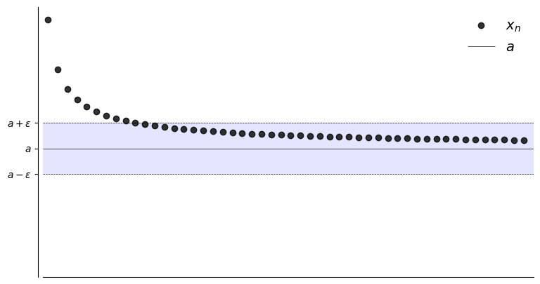
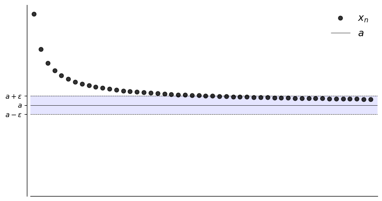
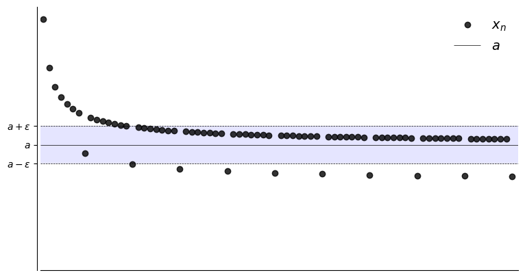
Suppose, for any \(\epsilon > 0\), we can find an \(N \in \mathbb{N}\) such that
Then \(\{x_n\}\) is said to converge to \(a\)
Convergence to \(a\) in symbols,
expression \(| x_n -a | <\epsilon\) defines an \(\epsilon\)-neighborhood around \(a\)
The sequence \(\{x_n\}\) is eventually in this \(\epsilon\)-neighborhood around \(a\)
Show code cell source
import matplotlib.pyplot as plt
import numpy as np

# from matplotlib import rc
# rc('font',**{'family':'serif','serif':['Palatino']})
# rc('text', usetex=True)

def fx(n):
    return 1 + 1/(n**(0.7))
def subplots(fs):
    "Custom subplots with axes throught the origin"
    fig, ax = plt.subplots(figsize=fs)
    # Set the axes through the origin
    for spine in ['left', 'bottom']:
        ax.spines[spine].set_position('zero')
    for spine in ['right', 'top']:
        ax.spines[spine].set_color('none')
    return fig, ax
def plot_seq(N,epsilon,a,fn):
    fig, ax = subplots((9, 5))
    xmin, xmax = 0.5, N+1
    ax.set_xlim(xmin, xmax)
    ax.set_ylim(0, 2.1)
    n = np.arange(1, N+1)
    ax.set_xticks([])
    ax.plot(n, fn(n), 'ko', label=r'$x_n$', alpha=0.8)
    ax.hlines(a, xmin, xmax, color='k', lw=0.5, label='$a$')
    ax.hlines([a - epsilon, a + epsilon], xmin, xmax, color='k', lw=0.5, linestyles='dashed')
    ax.fill_between((xmin, xmax), a - epsilon, a + epsilon, facecolor='blue', alpha=0.1)
    ax.set_yticks((a - epsilon, a, a + epsilon))
    ax.set_yticklabels((r'$a - \epsilon$', r'$a$', r'$a + \epsilon$'))
    ax.legend(loc='upper right', frameon=False, fontsize=14)
    plt.show()

N = 50
a = 1
plot_seq(N,0.30,a,fx)
plot_seq(N,0.20,a,fx)
plot_seq(N,0.10,a,fx)
Definition
The point \(a\) is called the limit of the sequence, denoted
if
Example
\(\{x_n\}\) defined by \(x_n = 1 + 1/n\) converges to \(1\):
To prove this we must show that \(\forall \, \epsilon > 0\), there is an \(N \in \mathbb{N}\) such that
To show this formally we need to come up with an “algorithm”
You give me any \(\epsilon > 0\)
I respond with an \(N\) such that equation above holds
In general, as \(\epsilon\) shrinks, \(N\) will have to grow
Proof:
Here’s how to do this for the case \(1 + 1/n\) converges to \(1\)
First pick an arbitrary \(\epsilon > 0\)
Now we have to come up with an \(N\) such that
Let \(N\) be the first integer greater than \( 1/\epsilon\)
Then
Remark: Any \(N' > N\) would also work
Example
The sequence \(x_n = 2^{-n}\) converges to \(0\) as \(n \to \infty\)
Proof:
Must show that, \(\forall \, \epsilon > 0\), \(\exists \, N \in \mathbb{N}\) such that
So pick any \(\epsilon > 0\), and observe that
Hence we take \(N\) to be the first integer greater than \(- \ln \epsilon / \ln 2\)
Then
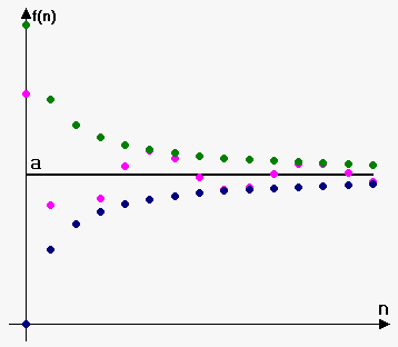
What if we want to show that \(x_n \to a\) fails?
To show convergence fails we need to show the negation of
In words, there is an \(\epsilon > 0\) where we can’t find any such \(N\)
That is, for any choice of \(N\) there will be \(n>N\) such that \(x_n\) jumps to the outside \(\epsilon\)-neighborhood around \(a\)
In other words, there exists a \(\epsilon\) such that \(|x_n-a| \geqslant \epsilon\) again and again as \(n \to \infty\).
This is the kind of picture we’re thinking of
Show code cell source
def fx2(n):
    return 1 + 1/(n**(0.7)) - 0.3 * (n % 8 == 0)

N = 80
a = 1
plot_seq(N,0.15,a,fx2)
Example
The sequence \(x_n = (-1)^n\) does not converge to any \(a \in \mathbb{R}\)
Proof:
This is what we want to show
Since it’s a “there exists”, we need to come up with such an \(\epsilon\)
Let’s try \(\epsilon = 0.5\), so that the \(\epsilon\)-neighborhood around \(a\) is
We have:
If \(n\) is odd then \(x_n = -1\) when \(n > N\) for any \(N\).
If \(n\) is even then \(x_n = 1\) when \(n > N\) for any \(N\).
Therefore even if \(a=1\) or \(a=-1\), \(\{x_n\}\) is not in \((a-0.5, a+0.5 )\) infinitely many times as \(n \to \infty\).
It holds for all other values of \(a \in \mathbb{R}\) as well
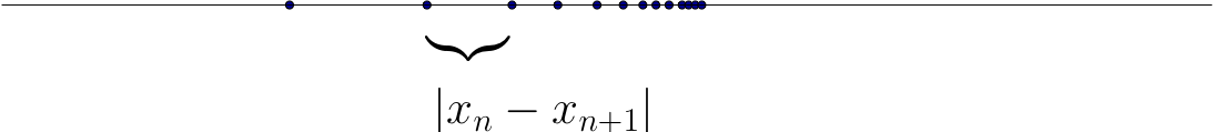
Cauchy sequences#
Informal definition: Cauchy sequences are those where \(|x_n - x_{n+1}|\) gets smaller and smaller
Example
Sequences generated by iterative methods for solving nonlinear equations often have this property
Definition
A sequence \(\{x_n\}\) is called Cauchy if
Alternatively
Cauchy sequences allow to establish convergence without finding the limit itself!
Fact
Every convergent sequence is Cauchy, and every Cauchy sequence is convergent.
Proof
Proof of \(\Rightarrow\):
Let \(\{x_n\}\) be a sequence converging to some \(a \in \mathbb{R}\)
Fix \(\epsilon > 0\)
We can choose \(N\) s.t.
For this \(N\) we have \(n \geq N\) and \(j \geq 1\) implies
Proof of \(\Leftarrow\):
Follows from the density property of \(\mathbb{R}\)
Example
\(\{x_n\}\) defined by \(x_n = \alpha^n\) where \(\alpha \in (0, 1)\) is Cauchy
Proof:
For any \(n , j\) we have
Fix \(\epsilon > 0\)
We can show that \(n > \log(\epsilon) / \log(\alpha) \implies \alpha^n < \epsilon\)
Hence any integer \(N > \log(\epsilon) / \log(\alpha)\) the sequence is Cauchy by definition.
Sub-sequences#
Let \(g: \mathbb{N} \rightarrow \mathbb{N}\) be an increasing mapping of the form \(g(k) = n_k\).
This means that \(g(k + 1) = n_{k+1} > n_k = g(k)\) for all \(k \in \mathbb{N}\).
The mapping \(f: \mathbb{N} \rightarrow X\) is a sequence from \(X\), and so is the mapping \(h: \mathbb{N} \rightarrow X\) given by \(h = f \circ g\)!
Note that \(h(k) = f(g(k)) = f(n_k)\).
\(f\) generates the sequence \(\{x_1, x_2, \dots , x_{n_1 − 1}, x_{n_1} , x_{n_1 + 1}, \dots , x_{n_2 − 1}, x_{n_2}, x_{n_2 + 1}, \dots \}\)
\(h\) generates the sequence \(\{x_{n_1} , x_{n_2} , \dots \}\)
Definition
The sequence \(\{x_{n_k} \}_{n_k \in \mathbb{N}}\) where \(k \in \mathbb{N}\) and \(n_{k+1} > n_k\) for all \(k\), is referred to as a sub-sequence of the sequence \(\{ x_n \}_{n \in \mathbb{N}}\)
Note that every term in the sequence \(\{ x_{n_k} \}_{n_k \in \mathbb{N}}\) is found somewhere in the sequence \(\{ x_n \}_{n \in \mathbb{N}}\)
Note also that the (relative) order in which the terms appear is the same for each of the sequences (due to the fact that \(n_{k+1} > n_k\) for all \(k\))
Example
Consider the sequence \(\{ x_n \}_{n \in \mathbb{N}}\) where \(x_n = \frac{1}{n}\).
The mapping for this sequence is \(f(n) = \frac{1}{n}\).
The sequence looks like \(\left\{1, \frac{1}{2}, \frac{1}{3} , \dots , \frac{1}{n}, \dots \right\}\).
Consider the increasing mapping \(g: \mathbb{N} \rightarrow \mathbb{N}\) defined by \(g(k) = k^2\).
This, along with \(f\), generates the sub-sequence mapping
The associated sub-sequence is
Consider the increasing map \(g: \mathbb{N} \rightarrow \mathbb{N}\) defined by \(g(k) = 2^k\).
This, along with \(f\), generates the sub-sequence map
The associated sub-sequence is
Fact
If \(\{ x_n \}\) converges to \(x\) in \(\mathbb{R}\), then every subsequence of \(\{x_n\}\) also converges to \(x\)
Fact
If two different subsequences of a sequence converge to different limits, the original sequence is not convergent.
Examples for practice: do sequences converge?
Example
Example
Example
Example
Example
Example
Example
Example
Example
Example
Example
The sequence \(\left\{ \frac{1}{n} \right\}_{n \in \mathbb{N}}\) converges to the point \(x = 0\).
The sequence \(\left\{ \frac{1}{n^2} \right\}_{n \in \mathbb{N}}\) converges to the point \(x = 0\).
Recall that \(\left\{ \frac{1}{n^2} \right\}_{n \in \mathbb{N}}\) is a sub-sequence of \(\left\{ \frac{1}{n} \right\}_{n \in \mathbb{N}}\)
The sequence \(\left\{ \frac{1}{2^n} \right\}_{n \in \mathbb{N}}\) converges to the point \(x = 0\).
Recall that \(\left\{ \frac{1}{2^n} \right\}_{n \in \mathbb{N}}\) is a sub-sequence of \(\left\{ \frac{1}{n} \right\}_{n \in \mathbb{N}}\)
The sequence \(\left\{ \frac{(−1)^n}{n} \right\}_{n \in \mathbb{N}} = \{ −1, \frac{1}{2}, \frac{−1}{3} , \dots \}\) converges to the point \(x = 0\).
The sequence \(\left\{ \frac{n}{n + 1} \right\}_{n \in \mathbb{N}} = \{ \frac{1}{2}, \frac{2}{3}, \frac{3}{4}, \dots \}\) converges to the point \(x = 1\).
The sequence \(\{ (−1)^n \}_{n \in \mathbb{N}} = \{ −1, 1, −1, 1, \dots \}\) does not converge.
The sequence \(\{ n \}_{n \in \mathbb{N}}\) does not converge.
The sequence \(\left\{ ( \frac{1}{n} , \frac{(n−1)}{n} ) \right\}_{n \in \mathbb{N}}\) converges to \((0, 1)\).
The sequence \(\left\{ ( \frac{(−1)^n}{n}, \frac{(−1)^n}{n} ) \right\}_{n \in \mathbb{N}}\) converges to \((0, 0)\).
The sequence \(\{ ((−1)^n, (−1)^n) \}_{n \in \mathbb{N}}\) does not converge.
The sequence \(\{ (n, n) \}_{n \in \mathbb{N}}\) does not converge.
Properties of limits#
Fact
\(x_n \to a\) in \(\mathbb{R}\) if and only if \(|x_n - a| \to 0\) in \(\mathbb{R}\)
If \(x_n \to x\) and \(y_n \to y\) then \(x_n + y_n \to x + y\)
If \(x_n \to x\) and \(\alpha \in \mathbb{R}\) then \(\alpha x_n \to \alpha x\)
If \(x_n \to x\) and \(y_n \to y\) then \(x_n y_n \to xy\)
If \(x_n \to x\) and \(y_n \to y\) then \(x_n / y_n \to x/y\), provided \(y_n \ne 0\), \(y \ne 0\)
If \(x_n \to x\) then \(x_n^p \to x^p\)
Proof
Let’s prove that
\(x_n \to a\) in \(\mathbb{R}\) means that
\(|x_n - a| \to 0\) in \(\mathbb{R}\) means that
Obviously equivalent
Exercise: Prove other properties using definition of limit
Fact
Each sequence in \(\mathbb{R}\) has at most one limit
Proof
Proof for the \(\mathbb{R}\) case.
Suppose instead that \(x_n \to a \text{ and } x_n \to b \text{ with } a \ne b \)
Take disjoint \(\epsilon\)-neighborhoods around \(a\) and \(b\) as shown
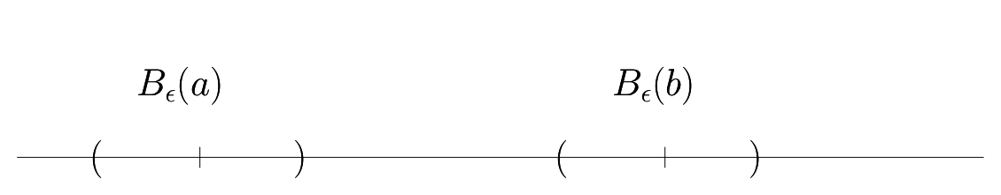
Since \(x_n \to a\) and \(x_n \to b\),
\(\exists \; N_a\) s.t. \(n \geq N_a \implies |x_n -a|<\epsilon\)
\(\exists \; N_b\) s.t. \(n \geq N_b \implies |x_n -b|<\epsilon\)
But then \(n \geq \max\{N_a, N_b\} \implies \) \(|x_n -a|<\epsilon\) and \(|x_n -b|<\epsilon\)
Contradiction, as the intervals around \(a\) and \(b\) are assumed disjoint
Fact
Weak inequalities are preserved in the limit.
Example
Find limit of \(x_n = \tfrac{1}{n} \Big( \sin(n^2-n+\exp(n)) +1 \Big)\) as \(n \to \infty\)
Solution: note that \(\sin(\cdot) \in [-1,1]\), and therefore the expression in brackets lies on the interval \([0,2]\). We have
Thus, \(0 \leqslant \lim_{n \to \infty} x_n \leqslant 0\), and so \(\lim_{n \to \infty} x_n = 0\)
Fact (Squeeze theorem)
Let \(x_n, y_n, z_n\) be sequences in \(\mathbb{R}\) such that \(x_n \leqslant y_n \leqslant z_n\) for all \(n>N\) for some \(N \in \mathbb{N}\), and suppose that \(x_n \to A\) and \(z_n \to A\) as \(n \to \infty\). Then \(y_n \to A\) as \(n \to \infty\).
Proof
See the intuition for the proof at Math Stack Exchange
Euler’s constant \(e\)#
Euler’s constant, which is usually denoted by \(e\), is an irrational number that is defined as the limit of a particular sequence of rational numbers.
Consider the sequence
This sequence converges to Euler’s constant. Euler’s constant is defined to be
Computing Euler’s constant as a limit of a sequence
e0 = 2.71828182845904523536028747135266
f = lambda n: (1+1/n)**n
print('Approximation of Euler constant')
for i in range(0,10100,500):
    e = f(i+1)
    print('iter = {:5d}: e = {:14.8f} err = {:14.10f}'.format(i,e,e0-e))
Approximation of Euler constant
iter =     0: e =     2.00000000 err =   0.7182818285
iter =   500: e =     2.71557393 err =   0.0027079019
iter =  1000: e =     2.71692529 err =   0.0013565409
iter =  1500: e =     2.71737689 err =   0.0009049376
iter =  2000: e =     2.71760291 err =   0.0006789198
iter =  2500: e =     2.71773859 err =   0.0005432399
iter =  3000: e =     2.71782907 err =   0.0004527577
iter =  3500: e =     2.71789372 err =   0.0003881134
iter =  4000: e =     2.71794221 err =   0.0003396225
iter =  4500: e =     2.71797993 err =   0.0003019027
iter =  5000: e =     2.71801010 err =   0.0002717240
iter =  5500: e =     2.71803480 err =   0.0002470304
iter =  6000: e =     2.71805538 err =   0.0002264511
iter =  6500: e =     2.71807279 err =   0.0002090370
iter =  7000: e =     2.71808772 err =   0.0001941098
iter =  7500: e =     2.71810066 err =   0.0001811725
iter =  8000: e =     2.71811198 err =   0.0001698519
iter =  8500: e =     2.71812197 err =   0.0001598629
iter =  9000: e =     2.71813084 err =   0.0001509835
iter =  9500: e =     2.71813879 err =   0.0001430386
iter = 10000: e =     2.71814594 err =   0.0001358880
See an excellent video about the Euler constant by Numberphile YouTube
Important notational comment
We have been looking at sequences drawn from some set \(X\). The \(n\)-th element of such a sequence was denoted by \(x_n\). This requires that \(x_n \in X\).
Do not confuse this \(x_n\) with the \(n\)-th coordinate of the point \(x = (x_1, x_2, \dots , x_{(n−1)}, x_n, x_{(n+1)}, \dots , x_L) \in \mathbb{R}^L\).
If we are considering sequences of points (or vectors) in \(\mathbb{R}^L\), then we might want to use superscripts to denote sequence position and subscripts to denote coordinates.
In this way, the \(k\)-th element of the sequence \(\{ x_n \}^\infty_{n=1}\) would be the point (or vector) \(x_k = (x^k_1, x^k_2, \dots , x^k_{(n−1)}, x^k_n, x^k_{(n+1)}, \dots , x^k_L)\). Note that the \(k\) in this case is an index, NOT a power.