📖 Multivariate differential calculus (part 2)

📖 Multivariate differential calculus (part 2)#

⏱ | words

Today we will continue our discussion of differential calculus of single-real-valued multivariate functions, \(f: X \subset \mathbb{R}^n \rightarrow Y \subset \mathbb{R}\).

We will be focussing on two concepts. These are implicit functions and homogenous functions.

Implicit functions#

Until now we have been working with explicit functions where the dependet variable, \(y\), is on the left side of the equation and the independet variables, \(x_i\), are on the right side

\[ y = f(x_1,x_2,\dots,x_n). \]

Frequently, we have to work with equations where the dependent variable cannot be separated from the independent variables

\[ G(x_1,x_2,\dots,x_n,y) = c. \]

We say that \(G(x_1,x_2,\dots,x_n,y) = c\) represent a relationship between \(y\) and \(x\) that defines an implicit function \(y\) of \(x\).

When dealing with implicit functions we want to know the following two answers:

Does \(G(x_1,x_2,\dots,x_n,y) = c\) determine \(y\) as a continuous implicit function of \((x_1,x_2,\dots,x_n)\)?
If so, how does changes in \(x\) affect \(y\)?

Example: The line of the cicle

The unit cicle has the representation

\[ x^2 + y^2 = 1. \]

Circle Line

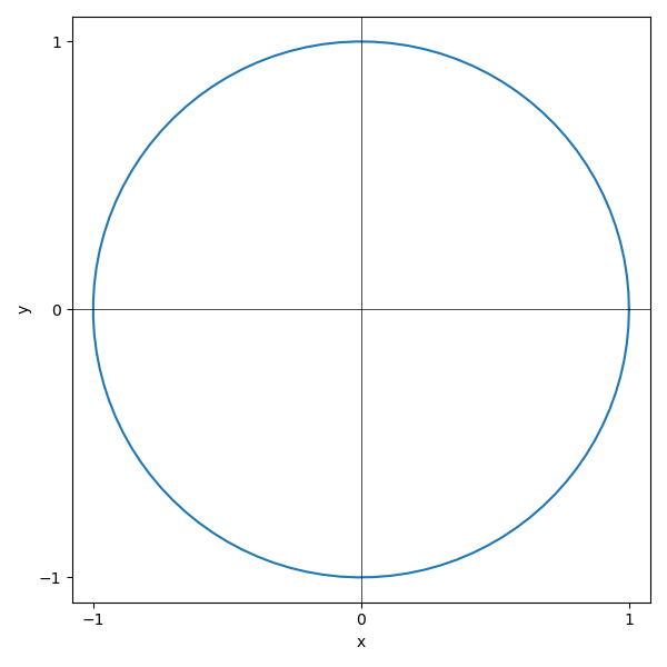
Consider the point \(x=0\), \(y=1\). In the neighborhood of this point \(y\) is an explicit function of \(x\)

\[ y(x) = \sqrt{x^2 - 1}. \]

\(y(x)\) can be represented by a different explicit function around the neighborhood at the point \(x=0\), \(y=-1\)

\[ y(x) = -\sqrt{x^2 - 1}. \]

In contrast, \(y\) cannot be represented by a well defined function around the points \((-1,0)\) and \((1,0)\).

Example: Polynomial equation of order five

Consider the polynomial equation

\[ y^5 + y^3 + y + x = 0. \]

\(x\) can be expressed as an explicit function of \(y\)

\[ x(y) = - y^5 - y^3 - y. \]

However, polynomials of order \(k \geq 5\) has no explicit solution. Hence, there exist no explicit function \(y\) of \(x\). Instead, the polynomial equation defines an implicit function for \(y\) of \(x\).

Suppose we could find a function \(y=y(x)\) which solves this equation for any \(x\)

\[ y(x)^5 + y(x)^3 + y(x) + x = 0. \]

Use the chain rule to find \(y'(x)\)

\[\begin{split} 5 y(x)^4 y'(x) + 3 y(x)^2 y'(x) + y'(x) + 1 = 0 \\ \Leftrightarrow y'(x) =-\frac{1}{5 y(x)^4 + 3 y(x)^2 + 1} \end{split}\]

The point \(x=-3\), \(y=1\) solves the polynomial equation, and

\[ y'(3)=-\tfrac{1}{5 + 3 + 1} = -\tfrac{1}{8} \]

We conclude that there exists an implicit function \(y=y(x)\) in the neighborhood around (-3,1) that solves polynomial equation and it is differentiable.

Now, let’s carry this computation out more generally for the implicit function \(G(x,y)=c\) around the specific point \(x=x^*\), \(y=y^*\), and let’s suppose there exist a solution \(y=y(x)\). Use the chain rule to differentiate wrt \(x\)

\[ \frac{\partial G\left(x^*, y(x^*)\right)}{\partial x} + \frac{\partial G\left(x^*, y(x^*)\right)}{\partial y} y'(x)=0. \]

Solving for \(y'(x)\) yields

\[ y'(x) =-\frac{\tfrac{\partial G\left(x^*, y(x^*)\right)}{\partial x} }{\tfrac{\partial G\left(x^*, y(x^*)\right)}{\partial y}}. \]

We see that if the solution \(y(x)\) of \(G(x,y)=c\) exists and is differentiable it is necessary that \(\partial G\left(x_0, y(x_0)\right) /\partial y\) be nonezero. The implicit function theorem stated below implies that this necessary condition is also a sufficient condition.

Fact (Implicit function theorem I)

Let \(G\left(x, y\right)\) be a \(C^1\) function around the point \((x^*,y^*)\) in \(\mathbb{R}^2\). Suppose \(G(x^*,y^*)=c\) and consider the expression

\[ G(x,y)=c. \]

If \(\partial G\left(x^*, y(x^*)\right) / \partial y \neq 0\), then there exists a \(C^1\) function \(y=y(x)\) defined in neighborhood around the point \(x^*\) such that

\(G(x,y(x)) = c\) for all \(x\) around \((x^*,y^*)\)
\(y(x^*)=y^*\)
the derivative of \(y\) wrt \(x\) at \((x^*,y^*)\) is

\[ y'(x) =-\frac{\tfrac{\partial G\left(x^*, y(x^*)\right)}{\partial x} }{\tfrac{\partial G\left(x^*, y(x^*)\right)}{\partial y}}. \]

The implicit function theorem provides conditions under which a relationship of the form \(G(x,y)=c\) implies that there exists a implicit function \(y=y(x)\) locally.

Example: The line of the cicle

When the implicit function theorem is applied to the line of the circle we get that

\[\begin{split} y'(x) &= -\frac{\tfrac{\partial y^2 + x^2}{\partial x}}{\tfrac{\partial y^2 + x^2}{\partial y}} \\ &= -\frac{2x}{2y} \\ &= -\frac{x}{y} \end{split}\]

which is not defined in the point (-1,0) and (1,0) .

The implicit function theoriem can be extended to \(G(x_1,x_2,\dots,x_n)=c\).

Fact (Implicit function theorem II)

Let \(\mathbf{x}=(x_1,x_2,\dots,x_n)\) and \(G\left(\mathbf{x}, y\right)\) be a \(C^1\) function around the point \((\mathbf{x}^*,y^*)\) in \(\mathbb{R}^{n+1}\). Suppose \(G(\mathbf{x}^*,y^*)=c\) and consider the expression

\[ G(\mathbf{x},y)=c. \]

If \(\partial G\left(\mathbf{x}^*, y(\mathbf{x}^*)\right) / \partial y \neq 0\), then there exists a \(C^1\) function \(y=y(\mathbf{x})\) defined in the neighborhood around the point \(\mathbf{x}^*\) such that

\(G(\mathbf{x},y(\mathbf{x})) = c\) for all \(\mathbf{x}\) around \((\mathbf{x}^*,y^*)\)
\(y(\mathbf{x}^*)=y^*\)
for each \(i\) the derivative of \(y\) wrt \(x_i\) is

\[ \frac{\partial y(\mathbf{x}^*)}{\partial x_i} = -\frac{\tfrac{\partial G\left(\mathbf{x}^*,y^*\right)}{\partial x_i} }{\tfrac{\partial G\left(\mathbf{x}^*,y^*\right)}{\partial y}}. \]

Example: \(G(x,y,z)=c\)

Consider the relationship

\[ - 3 x^2 y + y z - 4 x z = 7. \]

We will show that near \((-1,1,2)\) we can write \(y=y(x,z)\) and we will find the partial \(\partial y / \partial x\) to that point

\[ - 3 \cdot (-1)^2 \cdot 1 + 1 \cdot 2 - 4 \cdot (-1) \cdot 2 = - 3 + 2 + 8 = 7 \]

Find the partial derivatives of \(G\) with respect to \(y\) and \(x\)

\[\begin{split} \frac{\partial G}{\partial x} &= -6xy - 4z. \\ \frac{\partial G}{\partial y} &= -3x^2 + z. \end{split}\]

The partial derivative is given by the implicit function theorem as

\[ \frac{\partial y}{\partial x} = -\frac{\tfrac{\partial G}{\partial x} }{\tfrac{\partial G}{\partial y}} = -\frac{-6xy - 4z}{-3x^2 + z} \]

We conclude that there exists a \(C^1\) function \(y=y(x,z)\) in the neighborhood around the point (-1,1,2).

Level sets#

Level curves can be used to visualize single-real-valued bivariate functions, \(f: X \subset \mathbb{R}^2 \rightarrow Y \subset \mathbb{R}\).

Fact (Level curve)

A curve \(\ell\) in \(\mathbb{R}^2\) is called a level curve of \(y=f(x_1,x_2)\) if the value of \(f\) on every point of \(\ell\) is some fixed \(c\).

Example: Level curve

\(x^2 + y^2 = c\) is the level curve of \(z=x^2 + y^2\).

Similarly, level surfaces can be used to visualize single-real-valued trivariate functions, \(f: X \subset \mathbb{R}^3 \rightarrow Y \subset \mathbb{R}\).

Fact (Level surface)

A surface \(S\) in \(\mathbb{R}^3\) is called a level surface of \(f(x_1,x_2,x_3)\) if the value of \(f\) on every point of \(S\) is some fixed \(c\).

Example: Level surface

\(x^2 + y^2 - z = c\) is the level surface of \(w=x^2 + y^2 - z\).

This can of course be generalized to higher order functions, \(f: X \subset \mathbb{R}^n \rightarrow Y \subset \mathbb{R}\)

Fact (Level sets)

A manifold \(M\) in \(\mathbb{R}^n\) is called a level set of \(f(x_1,x_2,\dots,x_n)\) if the value of \(f\) on every point of \(M\) is some fixed \(c\).

The slope of an isoquant curve#

Suppose that \(f: \mathbb{R}_{+}^{2} \rightarrow \mathbb{R}_{+}\) is a production function.

\[ Q = f(K,L). \]

The level curve of the production function represent a relationship between the capital (K) and labor (L) inputs that keeps the production constant at \(c\)

\[ f(K,L) = c. \]

Given the specified production function we might be able to find an explicit or implicit function for the isoquant curve, \(L=L(K)\). In both cases we can use the implicit function theorem to calculate the slope of the isoquant curve.

\[\begin{split} \frac{\partial f(K,L)}{\partial K} + \frac{\partial f(K,L)}{\partial L} \frac{\partial L(K)}{\partial K} = 0 \\ \Leftrightarrow \frac{\partial L(K)}{\partial K} = -\frac{\tfrac{\partial f(K,L)}{\partial K}}{\tfrac{\partial f(K,L)}{\partial L}} \end{split}\]

The slope of the isoquant curve is referred to as the marginal rate of technical substitution

\[ \text{MRTS}_{LK} = -\frac{\tfrac{\partial f(K,L)}{\partial K}}{\tfrac{\partial f(K,L)}{\partial L}}. \]

It measures how much of one input would be needed to compensate for a one-unit loss of the other while keeping the production at the same level.

Marginal rate of technical substitution between input \(x_i\) and \(x_j\) of a multivariate function is defined as

\[ \text{MRTS}_{x_i,x_j} = -\frac{\tfrac{\partial f(x_1,x_2,\dots,x_n)}{\partial x_j}}{\tfrac{\partial f(x_1,x_2,\dots,x_n)}{\partial x_i}}. \]

Example: \(f(K,L,T)=c\)

Consider the level surface of the Cobb-Douglas function of three inputs (capital, labor, and land)

\[ A C^{\alpha} L^{\beta} T^{\delta} = c \]

Calculate the marginal rate of substitution between capital and labor

\[\begin{split} \alpha A C^{\alpha-1} L^{\beta} T^{\delta} \frac{\partial C(L,T)}{\partial L} + \beta A C^{\alpha} L^{\beta-1} T^{\delta} = 0 \\ \Leftrightarrow \frac{\partial C(L,T)}{\partial L} = -\frac{\beta A C^{\alpha} L^{\beta-1} T^{\delta}}{\alpha A C^{\alpha-1} L^{\beta} T^{\delta}} = \frac{\beta}{\alpha} \frac{C}{L} \end{split}\]

Calculate the marginal rate of substitution between capital and land

\[\begin{split} \alpha A C^{\alpha-1} L^{\beta} T^{\delta} \frac{\partial C(L,T)}{\partial T} + \delta A C^{\alpha} L^{\beta} T^{\delta-1} = 0 \\ \Leftrightarrow \frac{\partial C(L,T)}{\partial L} = -\frac{\delta A C^{\alpha} L^{\beta} T^{\delta-1}}{\alpha A C^{\alpha-1} L^{\beta} T^{\delta}} = \frac{\delta}{\alpha} \frac{C}{T} \end{split}\]

Calculate the marginal rate of substitution between labor and land

\[\begin{split} \beta A C^{\alpha} L^{\beta-1} T^{\delta}\frac{\partial L(C,T)}{\partial T} + \delta A C^{\alpha} L^{\beta} T^{\delta-1} = 0 \\ \Leftrightarrow \frac{\partial L(C,T)}{\partial T} = -\frac{\delta A C^{\alpha} L^{\beta} T^{\delta-1}}{\beta A C^{\alpha} L^{\beta-1} T^{\delta}} = \frac{\delta}{\beta} \frac{L}{T} \end{split}\]

Homogeneous functions#

Consider a function \(f: S \longrightarrow \mathbb{R}\), where \(S \subseteq \mathbb{R}^{n}\). Let \(\lambda>0\) be a positive real number.

Definition

The function \(f\left(x_{1}, x_{2}, \cdots, x_{n}\right)\) is said to be homogeneous of degree \(r\) if

\[ f\left(\lambda x_{1}, \lambda x_{2}, \cdots, \lambda x_{n}\right)=\lambda^{r} f\left(x_{1}, x_{2}, \cdots, x_{n}\right) \]

for all \(\left(x_{1}, x_{2}, \cdots, x_{n}\right) \in S\) and all \(\lambda>0\).

Example

The function

\[ 3x^5 y + 2x^2 y^4 - 3 x^3 y^3, \]

is homogenous of degree 6

\[\begin{split} 3(\lambda x)^5 (\lambda y) + 2(\lambda x)^2 (\lambda y)^4 - 3 (\lambda x)^3 (\lambda y)^3 &= 3\lambda^5 x^5 \lambda y + 2\lambda^2 x^2 \lambda^4 y^4 - 3 \lambda^3 x^3 \lambda^3 y^3 \\ &= 3\lambda^6 x^5 y + 2\lambda^6 x^2 y^4 - 3 \lambda^6 x^3 y^3 \\ &= \lambda^6 \left(3 x^5 y + 2 x^2 y^4 - 3 x^3 y^3 \right). \end{split}\]

The function

\[ 3x^{3/4} y^{1/4} + 6x + 4, \]

is not homogenous

\[ 3(\lambda x)^{3/4} (\lambda y)^{1/4} + 6(\lambda x) + 4 = 3 \lambda x^{3/4} y^{1/4} + 6\lambda x + 4. \]

Definition

A function that is homogeneous of degree one is said to be linearly homogeneous.

Definition

Let \(z=f(x)\) be a \(C^1\) function. If \(f\) is homogenous of degree \(r\), its first order partial derivatives are homogenous of degree \(r-1\).

By definition

\[ f(\lambda x_1, \lambda x_2, \dots, \lambda x_n) = \lambda^r f(x_1,x_2,\dots,x_n). \]

Use the chain rule wrt x_i on both sides of the equation

\[ \frac{\partial f(\lambda x_1, \lambda x_2, \dots, \lambda x_n)}{\partial x_i} \lambda = \lambda^r \frac{\partial f(x_1,x_2,\dots,x_n)}{\partial x_i}, \]

and divide both sides by \(\lambda\)

\[ \frac{\partial f(\lambda x_1, \lambda x_2, \dots, \lambda x_n)}{\partial x_i} = \lambda^{r-1} \frac{\partial f(x_1,x_2,\dots,x_n)}{\partial x_i}. \]

Fact

Let \(q=f(x)\) be a \(C^1\) homogenous function on \(\mathbb{R}^n_+\). The tangent planes to the level sets of \(f\) have constant slope along each ray from the origin.

Consider the homogenous production function on \(\mathbb{R}^2_+\). We want to show that the MRTS is constant along rays from the origin. Let \((\lambda L_0,\lambda K_0)=(L_1, K_1)\). The MRTS between input \(L\) and \(K\) at \((L_1, K_1)\) equals

\[\begin{split} \frac{f_{K}(L_1, K_1)}{f_{L}(L_1, K_1)} &= \frac{f_{K}(\lambda L_0,\lambda K_0)}{f_{L}(\lambda L_0,\lambda K_0)} \\ &= \frac{\lambda^{r-1} f_{K}( L_0, K_0)}{\lambda^{r-1} f_{L}( L_0, K_0)} \\ &= \frac{f_{K}(L_0, K_0)}{f_{L}( L_0, K_0)} \\ \end{split}\]

Euler’s theorem#

Fact (Euler’s theorem)

Suppose that the function \(f\left(x_{1}, x_{2}, \cdots, x_{n}\right)\) is homogeneous of degree \(r\). In this case we have

\[ \sum_{i=1}^{n} x_{i}\frac{\partial f}{\partial x_{i}}\left(\mathbf{x} \right)=r f\left(\mathbf{x}\right). \]

Recall the definition of a homogenous function of degree \(r\)

\[ f(\lambda \mathbf{x}) = \lambda^{r} f(\mathbf{x}). \]

Differentiate both sides wrt \(\lambda\)

\[ \sum_{i=1}^{n} x_{i}\frac{\partial f}{\partial x_{i}}\left(\lambda \mathbf{x} \right) = r \lambda^{r-1} f(\mathbf{x}). \]

Set \(\lambda=1\).

Returns to scale#

Suppose that an \(n\) input and one output production technology can be represented by a homogenous production function of the form

\[ Q=f\left(L_{1}, L_{2}, \cdots, L_{n}\right) . \]

The production technology is said to display:

constant returns to scale: \(f\left(\lambda L_{1}, \lambda L_{2}, \cdots, \lambda L_{n}\right)=\lambda Q\).
decreasing returns to scale: \(f\left(\lambda L_{1}, \lambda L_{2}, \cdots, \lambda L_{n}\right)<\lambda Q\).
increasing returns to scale: \(f\left(\lambda L_{1}, \lambda L_{2}, \cdots, \lambda L_{n}\right)>\lambda Q\).

Cobb-Douglas production functions#

Suppose that an two input and one output production technology can be represented by a production function of the form

\[ Q=f(L, K)=A L^{\alpha} K^{\beta} . \]

This type of production function is known as a Cobb-Douglas production function.

Suppose that \(\lambda>0\). Note that

\[\begin{split} \begin{aligned} f(\lambda L, \lambda K) & =A(\lambda L)^{\alpha}(\lambda K)^{\beta} \\ & =A \lambda^{\alpha} L^{\alpha} \lambda^{\beta} K^{\beta} \\ & =\lambda^{\alpha+\beta} A L^{\alpha} K^{\beta} \\ & =\lambda^{\alpha+\beta} f(L, K) \end{aligned} \end{split}\]

Thus we know that the Cobb-Douglas production function is homogeneous of degree \((\alpha+\beta)\).

If \((\alpha+\beta)<1\), then the Cobb-Douglas production function displays decreasing returns to scale;
If \((\alpha+\beta)=1\), then the Cobb-Douglas production function displays constant returns to scale; and
If \((\alpha+\beta)>1\), then the Cobb-Douglas production function displays increasing returns to scale.

Homothetict function#

Definition

Let \(I\) be an interval on the real line. Then, \(g: I \rightarrow \mathbb{R}\) is a monotonic transformation on \(I\) if \(g\) is a strictly increasing function on \(I\).

Definition

A function \(v: \mathbb{R}_{+}^n \rightarrow \mathbb{R}\) is called homothetic if it is a monotone transformation, \(g(z)\), of a homogenous function \(u: \mathbb{R}_{+}^n \rightarrow \mathbb{R}\)

\[ v(x) = g\left(u(\mathbf{x})\right) \]

for all \(\mathbf{x}\) in the domain.

Example: \(G(x,y,z)=c\)

The two functions

\[\begin{split} v_1(x,y)=x^3y^3 + xy \\ v_2(x,y)=xy + 1, \end{split}\]

are homothetic functions with \(u(x,y)=xy\) and the monotonic transformations

\[\begin{split} g_1(x,y) = z^3 + z \\ g_2(x,y) = z + 1, \end{split}\]

respectively.

Definition

Let \(u: \mathbb{R}_{+}^n \rightarrow \mathbb{R}\) be a strictly monotonic function. Then, \(u\) is a homothetic if and only if for all \(\mathbf{x}\) and \(\mathbf{y}\) in \(\mathbb{R}^n_+\),

\[ u(\mathbf{x}) \geq u(\mathbf{y}) \Leftrightarrow u(\alpha \mathbf{x}) \geq u(\alpha \mathbf{y}) \text{ for all } \alpha > 0. \]

Definition

Let \(u\) be a \(C^1\) function on \(\mathbb{R}^n_+\). If \(u\) is homothetic then the slopes of the tangent planes of the level sets of \(u\) are constant along each ray from the origin.

📖 Multivariate differential calculus (part 2)

Contents

📖 Multivariate differential calculus (part 2)#

Implicit functions#

Level sets#

The slope of an isoquant curve#

Homogeneous functions#

Euler’s theorem#

Returns to scale#

Cobb-Douglas production functions#

Homothetict function#