Announcements & Reminders

1. This week and the next week we have a guest lecturer

   Dr Esben Scriver Andersen

   • Office: 1018 HW Arndt Building

   • Email: esbenscriver.andersen@anu.edu.au

2. Online Test 4 on Monday May 6

   • will cover last two lectures:

     • linear systems of equations

     • multivariate differential calculus (part 1)

3. The final exam is scheduled!

   • Friday May 31, 2pm

   • 3 hours exam + 15 minutes reading time

   • closed book, no materials allowed

   • Manning Clark Hall, room 1.04, Cultural Centre Kambri

📖 Multivariate differential calculus (part 1)

⏱ | words

Sources and reading guide

[Sydsæter, Hammond, Strøm, and Carvajal, 2016]

Chapters 11 and 12 (pp. 407-494).

Introductory level references:

• [Bradley, 2008]: Chapter 7, Sections 1 to 3 (pp. 360-408).

• [Haeussler Jr and Paul, 1987]: Chapter 17, Sections 1 to 7 and Sections 9 to 10 (pp. 668-706 and 714-723).

• [Shannon, 1995]: Chapter 10, Sections 1 to 6 (pp. 450-489).

Intermediate mathematical economics textbooks:

• [Chiang, 1984]: Chapters 6-8 and Chapter 10 (pp. 127-227 and 268-306).

• [Chiang and Wainwright, 2005]: Chapters 6 to 10 (pp. 124-290).

• [Simon and Blume, 1994]: Chapters 2 to 5 (pp. 10-103).

Mathematics textbooks:

• [Spiegel, 1981]: Chapters 4, 6, 7 and 8; pp. 57-79 and 101-179.

• [Spiegel, 1981]: Chapters 3 and 4; pp. 35-81.

We want to extend our discussion of differential calculus from single-real-valued univariate functions, \(f(x_1)\), to single-real-valued multivariate functions, \(f(x_1,x_2,\dots,x_n)\).

We will be focussing on two concepts. These are partial derivatives and total derivatives.

Notation

To simplify notation we will sometimes denote vectors with bold letters, e.g. \(\mathbf{x}=(x_1,x_2,\dots,x_n)\). Hence, we can write our multivariate function as a function of a vector input, \(f(\mathbf{x})=f(x_1,x_2,\dots,x_n)\).

Single-real-valued multivariate functions

Definition

A single-real-valued multivariate function takes as input \(n\) real numbers and outputs a single real number,

\[ f: X \subseteq \mathbb{R}^{n} \rightarrow Y \subseteq \mathbb{R}. \]

Recall that:

• \(X\) is the domain of \(f\).

• \(Y\) is the target space of \(f\).

Often we simply write a single-real-valued multivariate functions as

\[ y = f(x_1,x_2,\dots,x_n), \]

where \(y\) is refered to as the dependent variable, and \(x_i\) is referred to as an independent variable. Alternatively, \(y\) and \(x_i\) can be referred to as the endogenous and exogenous variables, or the output and input variables.

Example

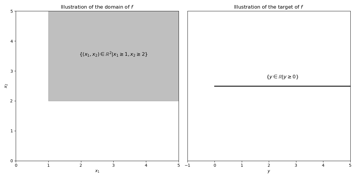
Consider the single-real-valued multivariate function \(f(x_1,x_2) = \sqrt{x_1 - 1} + \sqrt{x_2 - 2}\).

• the domain of \(f\) is \(\left\{ (x_1,x_2) \in \mathbb{R}^{2} | x_1 \geq 1, x_2 \geq 2 \right\}\).

• the target of \(f\) is \(\left\{ y \in \mathbb{R} | y \geq 0 \right\}\).

Fig. 33 Illustrations of domain and target of \(f\).

In economic analysis we will often use single-real-valued multivariate functions to represent

• production functions

• cost functions

• profit functions

• utility functions

• demand functions

Example

Important single-real-valued bivariate functions used in economic analysis:

• Linear function

\[f(\mathbf{x}) = a_{1} x_{1} + a_{2} x_{2}.\]

• Input-output function

\[f(\mathbf{x}) = \text{min}(a_1 x_1, a_2 x_2).\]

• Cobb-Douglas function

\[f(\mathbf{x}) = k x_{1}^{b_1} x_{2}^{b_2}.\]

• Constant elasticity of substitution (CES) function,

\[f(\mathbf{x}) = k (c_1 x_1^{a} + c_2 x_2^{a})^{b/a}.\]

These functions are straight forward to extent to more than two inputs.

Partial derivatives

Our primary goal in economic analysis is to understand how a change in one independent variable affect the dependent variable. By using partial derivatives we take the simplest approach by changing one variable at a time, keeping all other constant.

Definition

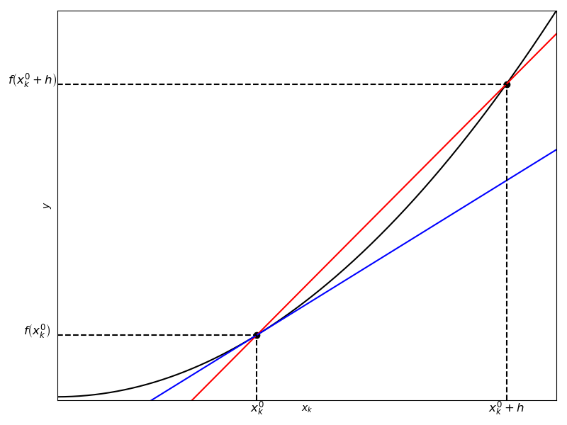
The partial derivative of the single-real-valued multivariate function \(f\) with respect to the variable \(x_{k}\) is defined as

\[ \begin{aligned} \frac{\partial f\left(\mathbf{x}\right)}{\partial x_{k}} = \lim _{h \rightarrow 0}\left\{\frac{f\left(x_{1}, \dots, x_{k} + h, x_{k+1}, \dots, x_n\right) - f\left(x_{1}, \dots, x_{k}, x_{k+1}, \dots, x_n\right)}{h}\right\} . \end{aligned} \]

Fig. 34 Illustration of the partial derivative with respect to \(x_k\).

Note that the partial derivative, \(\partial f\left(\mathbf{x}\right)/\partial x_k\), is a single-real-valued multivariate function itself, as it in general depend on all the independent variables.

As a matter of convenience partial derivatives are often denoted by \(f_{k}\left(\mathbf{x}\right)\) or \(f'_{k}\left(\mathbf{x}\right)\).

Definition

The gradient is defined as the vector of first-order partial derivatives of \(f\)

\[ \nabla f(\mathbf{x}) = \bigg(\tfrac{\partial f(\mathbf{x})}{\partial x_1}, \tfrac{\partial f(\mathbf{x})}{\partial x_1}, \dots, \tfrac{\partial f(\mathbf{x})}{\partial x_n} \bigg)^T \]

The gradient is commonly denoted by one of \(\nabla f(\mathbf{x}), D_{x} f(\mathbf{x})\), or \(\operatorname{grad} f(\mathbf{x})\).

Note that when calculating the partial derivative with respect \(x_k\) we treat the remaining independent variables as constants. Hence, we can use the same rules for partial differentiation as for differentiation of univariate functions.

Fact: Rules for partial differentiation

• \(f(\mathbf{x}) = c g(\mathbf{x}) \Rightarrow f_k\left( \mathbf{x} \right) = c g_k\left( \mathbf{x} \right)\).

• \(f(\mathbf{x}) = g(\mathbf{x}) + h(\mathbf{x}) \Rightarrow f_k\left( \mathbf{x} \right) = g_k\left( \mathbf{x} \right) + h_k\left( \mathbf{x} \right)\).

• \(f(\mathbf{x}) = g(\mathbf{x})h(\mathbf{x}) \Rightarrow f_k\left( \mathbf{x} \right) = g_k(\mathbf{x})h(\mathbf{x}) + g(\mathbf{x})h_k(\mathbf{x})\).

• \(f(\mathbf{x}) = g\left(h\left(\mathbf{x}\right)\right) \Rightarrow f_k\left( \mathbf{x} \right) = g_h\left(h\left(\mathbf{x}\right)\right)h_k\left(\mathbf{x}\right)\).

Example I

Consider the bivariate function \(y=f(x_1,x_2)=a x_1 + b x_2\). The partial derivative with respect to \(x_1\) is then

The partial derivative with respect to \(x_1\) is then

\[ f_1(x_1,x_2)=a. \]

The partial derivative with respect to \(x_2\) is then

\[ f_1(x_1,x_2)=b. \]

Example II

Consider the bivariate function \(y=f(x_1,x_2)=x_1 x_2\).

The partial derivative with respect to \(x_1\) is then

\[ f_1(x_1,x_2)=x_2. \]

The partial derivative with respect to \(x_2\) is then

\[ f_2(x_1,x_2)=x_1. \]

Definition

Some terminologi:

• If \(\partial f\left(\mathbf{x}\right)/\partial x_k\) exist for each \(k\), we say that \(f\) is differentiable at \(\mathbf{x}\).

• If these \(n\) partial derivative functions are continuous, we say that \(f\) is continously differentiable at \(\mathbf{x}\). This is denoted by \(f \in C^{1}\) on \(X\).

Some economic applications

Often in economic analysis the partial derivative has a straight forward interpretation

• production function: marginal product

• cost function: marginal cost

• profit function: marginal profit

• utility function: marginal utility

• demand function: marginal change in demand

Marginal products of production inputs

Suppose a firm’s production is described by a Cobb-Douglas production function, where labor (L) and capital (K) are the inputs:

\[ Q = f(L, K)=A L^{\alpha} K^{\beta} . \]

The marginal product of labour is simply the partial derivative with respect to labor. Thus we have

\[\begin{split} \begin{aligned} M P_{L}(L, K) & =\frac{\partial f(L, K)}{\partial L} \\ & =\frac{\partial\left(A L^{\alpha} K^{\beta}\right)}{\partial L} \\ & =\alpha A L^{\alpha-1} K^{\beta} \end{aligned} \end{split}\]

The marginal product of capital is simply the first-order derivative with respect to capital. Thus we have

\[\begin{split} \begin{aligned} M P_{K}(L, K) & =\frac{\partial f(L, K)}{\partial K} \\ & =\frac{\partial\left(A L^{\alpha} K^{\beta}\right)}{\partial K} \\ & =\beta A L^{\alpha} K^{\beta-1} \end{aligned} \end{split}\]

Elasticities

An elasticity measure the fractional response of the dependent variable, \(y=f(x_1,x_2,\dots,x_n)\), to a fractional change in an independent variable, e.g. \(x_k\), which can be written as

\[\begin{split} \varepsilon_{x_{k}} &= \left(\frac{f(x_1,\dots,x_k + h, x_{k+1},\dots,x_n) - f(x_1,\dots,x_k, x_{k+1},\dots,x_n)}{f(x_1,\dots,x_k, x_{k+1},\dots,x_n)} \right) / \left( \frac{h}{x_k} \right), \\ &= \frac{f(x_1,\dots,x_k + h, x_{k+1},\dots,x_n) - f(x_1,\dots,x_k, x_{k+1},\dots,x_n)}{h}\frac{x_k}{f(x_1,\dots,x_k, x_{k+1},\dots,x_n)}, \end{split}\]

where \(h\) is the change in \(x_k\). As \(h \rightarrow 0\), we can write this in terms of the partial derivative

\[ \varepsilon_{x_{k}} = \frac{\partial f(\mathbf{x})}{\partial x_k} \frac{x_k}{f(\mathbf{x})}. \]

Similar to partial derivatives, elasticities measure how sensitive the dependent variable is to changes in the independent variables. Unlike partial derivatives elasticities are unit-free.

Elasticities of production with respect to inputs

Suppose a firm production is described by a Cobb-Douglas production function:

\[ f(L, K)=A L^{\alpha} K^{\beta} . \]

We know from earlier that the partial derivatives of the Cobb-Douglas production function are

\[\begin{split} \frac{\partial f(L, K)}{\partial L} = \alpha A L^{\alpha-1} K^{\beta}. \\ \frac{\partial f(L, K)}{\partial K} = \beta A L^{\alpha} K^{\beta-1}. \\ \end{split}\]

Insert the partial derivate with respect to labor into the definition of elasticities

\[\begin{split} \varepsilon_{L} &= \tfrac{\partial f(L,K)}{\partial L}\tfrac{L}{f(L,K)}, \\ &= \alpha A L^{\alpha-1} K^{\beta}\frac{L}{A L^{\alpha} K^{\beta}}, \\ &= \alpha. \end{split}\]

Insert the partial derivate with respect to capital into the definition of elasticities

\[\begin{split} \varepsilon_{K} &= \tfrac{\partial f(L,K)}{\partial L}\tfrac{L}{f(L,K)}, \\ &= \beta A L^{\alpha} K^{\beta-1}\frac{K}{A L^{\alpha} K^{\beta}}, \\ &= \beta. \end{split}\]

Elasticities of demand

Suppose that an individual’s demand function for commodity \(k\) is given by

\[ D_{k}\left(\mathbf{p},y\right) = D_{k}\left(p_{1}, p_{2}, \dots, p_{n}, y\right), \]

where \(p_{i}\) is the price of commodity \(i\) and \(y\) is the consumer’s income.

• The own-price elasticity of demand for commodity \(k\) for this consumer is

\[ \begin{aligned} \varepsilon_{k}^{k}\left(\mathbf{p},y\right) & =\left(\frac{p_{k}}{D_{k}\left(\mathbf{p},y\right)}\right)\left(\frac{\partial D_{k}\left(\mathbf{p},y\right)}{\partial p_{k}}\right) . \end{aligned} \]

• The cross-price elasticity of demand for commodity \(k\) with respect to the price of commodity \(l\) for this consumer is

\[ \begin{aligned} \varepsilon_{l}^{k}\left(\mathbf{p},y\right) & =\left(\frac{p_{l}}{D_{k}\left(\mathbf{p},y\right)}\right)\left(\frac{\partial D_{k}\left(\mathbf{p},y\right)}{\partial p_{l}}\right). \end{aligned} \]

• The income elasticity of demand for commodity \(k\) for this consumer is

\[ \begin{aligned} \varepsilon_{y}^{k}\left(\mathbf{p},y\right) & =\left(\frac{y}{D_{k}\left(\mathbf{p},y\right)}\right)\left(\frac{\partial D_{k}\left(\mathbf{p},y\right)}{\partial y}\right) . \end{aligned} \]

We can use these elasticities to classify the types of commodities that are being considered:

• If \(\varepsilon_{y}^{k}>0\), then commodity \(k\) is a normal good.

• If \(\varepsilon_{y}^{k}<0\), then commodity \(k\) is an inferior good.

• If \(\varepsilon_{l}^{k}>0\), then commodities \(k\) and \(l\) are substitutes.

• If \(\varepsilon_{l}^{k}<0\), then commodities \(k\) and \(l\) are complements.

• The demand curve for most commodities will usually slope down. As such, we would usually expect \(\varepsilon_{k}^{k}<0\).

• However, there are circumstances in which the demand curve for a commodity can slope up over some range of prices (at least in theory). Such commodities are known as Giffen goods. In such circumstances, we would have \(\varepsilon_{k}^{k}>0\) over the relevant range of prices.

Second-order partial derivatives

Consider the function single-real-valued multivariate function \(f\left(x_1,x_2,\dots,x_n \right)\). Recall that if the first-order partial derivative exist it is also a single-real-valued multivariate function. The second-order partial derivative is given as the partial derivate of the first-order partial derivate

\[ \frac{\partial^{2} f\left(x_{1}, x_{2}, \dots, x_{n}\right)}{\partial x_{j} \partial x_{i}}=\frac{\partial}{\partial x_{j}}\left(\frac{\partial f\left(x_{1}, x_{2}, \dots, x_{n}\right)}{\partial x_{i}}\right), \]

where \(x_i\) is the input \(f\) is differentiated with respect to, and \(x_j\) is the input the first-order partial derivative is differentiated with respect to.

The second-order partial derivative is commonly denoted

\[ \frac{\partial^{2} f\left(x_{1}, x_{2}, \dots, x_{n}\right)}{\partial x_{j} \partial x_{i}}=f_{i j}\left(x_{1}, x_{2}, \dots, x_{n}\right) \]

Note again that if the second-order partial derivative exist it is also a single-real-valued multivariate function.

Definition

The Hessian is defined as the matrix of second-order partial derivatives of \(f\)

\[\begin{split} \nabla^2 f(\mathbf{x}) = \left(\begin{array}{cccc} \frac{\partial^{2} f(\mathbf{x})}{\partial x_{1}^{2}} & \frac{\partial^{2} f(\mathbf{x})}{\partial x_{2} \partial x_{1}} & \cdots & \frac{\partial^{2} f(\mathbf{x})}{\partial x_{n} \partial x_{1}} \\ \frac{\partial^{2} f(\mathbf{x})}{\partial x_{1} \partial x_{2}} & \frac{\partial^{2} f(\mathbf{x})}{\partial x_{2}^{2}} & \cdots & \frac{\partial^{2} f(\mathbf{x})}{\partial x_{n} \partial x_{2}} \\ \vdots & \vdots & \ddots & \vdots \\ \frac{\partial^{2} f(\mathbf{x})}{\partial x_{1} \partial x_{n}} & \frac{\partial^{2} f(\mathbf{x})}{\partial x_{2} \partial x_{n}} & \cdots & \frac{\partial^{2} f(\mathbf{x})}{\partial x_{n}^{2}} \end{array}\right) \end{split}\]

The Hessian is commonly denoted as \(H(\mathbf{x})\), \(\nabla^2 f(\mathbf{x})\), \(D_{xx^T}f(\mathbf{x})\), or \(\operatorname{hess} f(\mathbf{x})\).

The elements on the diagonal of the Hessian are referred to as second-order own partial derivatives, and the elements off the diagonal are referred to as second-order cross partial derivatives.

Definition

Some terminologi:

• If \(f\) is twice-differentiable at every point \(x \in X\), then \(f\) is said to be twice-differentiable on \(X\).

• If \(f\) is twice-differentiable on \(X\) and \(\frac{\partial^{2} f}{\partial x_{k} \partial x_{i}}\) is a continuous function on \(X\) for all combinations of \(i\) and \(j\) then \(f\) is said to be twice continuously differentiable on \(X\). This is denoted by \(f \in C^{2}\) on \(X\).

It is possible to extend the process of differentiation for multivariate functions to even higher orders than second-order derivatives. Doing so for partial derivatives is relatively straight-forward. However, this will not be done in this course.

Hessian of the Cobb-Douglas production function

Suppose that we have a Cobb-Douglas production function:

\[ f(L, K)=A L^{\alpha} K^{\beta} . \]

From earlier we know the partial derivatives of the Cobb-Douglas production function that constitute the gradient

\[\begin{split} \nabla f(\mathbf{x}) = \left(\begin{array}{c} \tfrac{\partial f(L,K)}{\partial L} \\ \tfrac{\partial f(L,K)}{\partial K} \end{array}\right) = \left(\begin{array}{c} \alpha A L^{\alpha-1} K^{\beta} \\ \beta A L^{\alpha} K^{\beta-1} \end{array}\right). \end{split}\]

Take the partial derivatives of the marginal product of labor

\[\begin{split} \tfrac{\partial^2 f(L,K)}{\partial L \partial L} &= \tfrac{\partial}{\partial L} \left( \tfrac{\partial f(L,K)}{\partial L} \right) \\ &= \tfrac{\partial}{\partial L} \left( \alpha A L^{\alpha-1} K^{\beta}\right) \\ &= \alpha (\alpha-1) A L^{\alpha-2} K^{\beta} \\ \tfrac{\partial^2 f(L,K)}{\partial L \partial K} &= \tfrac{\partial}{\partial K} \left( \tfrac{\partial f(L,K)}{\partial L} \right) \\ &= \tfrac{\partial}{\partial K} \left( \alpha A L^{\alpha-1} K^{\beta}\right) \\ &= \alpha \beta A L^{\alpha-1} K^{\beta-1} \end{split}\]

Take the partial derivatives of the marginal product of capital

\[\begin{split} \tfrac{\partial^2 f(L,K)}{\partial K \partial L} &= \tfrac{\partial}{\partial L} \left( \tfrac{\partial f(L,K)}{\partial K} \right) \\ &= \tfrac{\partial}{\partial L} \left( \beta A L^{\alpha} K^{\beta-1}\right) \\ &= \alpha \beta A L^{\alpha-1} K^{\beta-1} \\ \tfrac{\partial^2 f(L,K)}{\partial K \partial K} &= \tfrac{\partial}{\partial K} \left( \tfrac{\partial f(L,K)}{\partial K} \right) \\ &= \tfrac{\partial}{\partial K} \left( \beta A L^{\alpha} K^{\beta-1}\right) \\ &= \beta (\beta - 1) A L^{\alpha} K^{\beta-2} \end{split}\]

We can now set up the Hessian of the Cobb-Douglas production function

\[\begin{split} \nabla^2 f(\mathbf{x}) = \left(\begin{array}{cc} \tfrac{\partial^2 f(L,K)}{\partial L \partial L} & \tfrac{\partial^2 f(L,K)}{\partial L \partial K} \\ \tfrac{\partial^2 f(L,K)}{\partial K \partial L} & \tfrac{\partial^2 f(L,K)}{\partial K \partial K} \end{array} \right) = \left(\begin{array}{cc} \alpha (\alpha-1) A L^{\alpha-2} K^{\beta} & \alpha \beta A L^{\alpha-1} K^{\beta-1} \\ \alpha \beta A L^{\alpha-1} K^{\beta-1} & \beta (\beta-1) A L^{\alpha} K^{\beta-2} \end{array} \right). \end{split}\]

Note that the Hessian is symmetric.

It turns out that the second-order cross partial derivatives are equal in general. This is known as Young’s theorem.

Fact (Young’s theorem)

Suppose that \(f(x_1,x_2,\dots,x_n)\) is a \(C^2\) on its domain, X. Then, for each pair of indices \(i\), \(j\),

\[ \frac{\partial^2 f (\mathbf{x})}{\partial x_i \partial x_j} = \frac{\partial^2 f (\mathbf{x})}{\partial x_j \partial x_i}. \]

Young’s theorem states that the order of differentiation does not matter for a \(C^2\) function. The result is trivially true when \(i=j\). This is the case of second-order own partial derivatives.

Total differentiation

When calculating the partial derivative of a function \(f\) with respect to \(x_i\), we only allow \(x_i\) to vary and keep all other variables constant. In contrast, when calculating the total derivative we allow all independent variables to vary

\[ df = \sum_{i=1}^n \frac{\partial f(\mathbf{x})}{\partial x_i}dx_i. \]

\(df\) is the total derivative of \(f\) with respect to the change \(\mathbf{dx}=(dx_1,dx_2,\dots,dx_n)\). Unlike the partial derivate the total derivate does not restrict the analysis to be local, i.e. \(dx_i \rightarrow 0\).

Example I

Consider the bivariate function \(y=f(x_1,x_2)=a x_1 + b x_2\). The total derivative with respect to \(x_1\) is then

\[ df=a dx_1 + b dx_2. \]

Example II

Consider the bivariate function \(y=f(x_1,x_2)=x_1 x_2\). The partial derivative with respect to \(x_1\) is then

\[ df=x_2 dx_1 + x_1 dx_2. \]

The total derivative, \(df\), can be thought of as a linear approximation of the change in \(f\) due to the change \(\mathbf{dx}\).

\[ df \approx f(\mathbf{x} + \mathbf{dx}) - f(\mathbf{x}). \]

Hence, we can use total differentiation to approximate \(f\) around the point \(\mathbf{x}^0\)

\[ f(\mathbf{x}^0 + \mathbf{dx}) \approx f(\mathbf{x}^0) + \sum_{i=1}^n \frac{\partial f(\mathbf{x}^0)}{\partial x_i}dx_i. \]

This is an example of a first order Taylor approximation.

The chain rule

Many economic models involve composition functions. These are functions of one or serveral variables in wich the variables are themselves functions of other basic variables.

E.g. many models of economic growth regard production as a function of capital and labor, both which are functions of time. For these models, we can apply the chain rule to analyze how production changes over time due to changes in labor and capital.

Fact (chain rule I)

When \(z=f(x_1,x_2,\dots,x_n)\) with \(x_i=g_i(t)\) for every \(i\), then

\[ \frac{dz}{dt} = \sum_{i=1}^n \frac{\partial z}{\partial x_i} \frac{dx_i}{dt} \]

As every variable, \(x_i\), depends on the basic variable, \(t\), a small change in \(t\) sets off a chain reaction. The sum of the individual contributions is called the total derivative and is denoted \(dz/dt\).

Calculating the growth rate of the production

The production of the economy is given by the Cobb-Douglas production function \(y=f(L(t),K(t))\) where the labor and capital inputs are both functions of time.

Labor and capital is accumulated at constant growth rates

\[\begin{split} \dot{L} \equiv \frac{dL}{dt} &= g_L L(t). \\ \dot{K} \equiv \frac{dK}{dt} &= g_K K(t). \\ \end{split}\]

Use chain rule to calculate how production changes over time

\[\begin{split} \frac{dy}{dt} &= \frac{\partial f(L,K)}{\partial L} \frac{dL}{dt} + \frac{\partial f(L,K)}{\partial K} \frac{dK}{dt} \\ &= \alpha A L^{\alpha-1} K^{\beta} g_L L + \beta A L^{\alpha} K^{\beta-1} g_K K \\ &= \alpha A L^{\alpha} K^{\beta} g_L + \beta A L^{\alpha} K^{\beta} g_K \\ &= (\alpha g_L + \beta g_K) y. \end{split}\]

Divide both sides with the production, \(y\)

\[ \frac{\dot{y}}{y} = \alpha g_L + \beta g_K. \]

The growth rate of the economy is constant, and is given by dot product of the elasticities and growth rates with respect to each of the production inputs.

The chain rule can be generalized by allowing the variables, \(x_i\), to be a function of more than one basic variable.

Fact (chain rule II)

When \(z=f(x_1,x_2,\dots,x_n)\) with \(x_i=g_i(t_1,t_2,...,t_m)\) for every \(i\), then

\[ \frac{\partial z}{\partial t_j} = \sum_{i=1}^n \frac{\partial z}{\partial x_i} \frac{\partial x_i}{\partial t_j} \]

for each \(j=1,2,\dots,m\)

Excercise

Calculate the partial derivatives and elasticities of the CES production function

The CES production function is given by:

\[ Y = A \left( aL^r + bK^r \right)^{\frac{s}{r}}. \]

The first order partial derivatives with respect to labor is:

\[\begin{split} \frac{\partial Y}{\partial L} &= \tfrac{s}{r} A \left( aL^r + bK^r \right)^{\frac{s}{r} - 1} arL^{r-1} \\ &= \frac{saL^{r}}{aL^r + bK^r} \frac{Y}{L} \\ \end{split}\]

The first order partial derivatives with respect to capital is:

\[\begin{split} \frac{\partial Y}{\partial K} &= \tfrac{s}{r} A \left( aL^r + bK^r \right)^{\frac{s}{r} - 1} brK^{r-1} \\ &= \frac{sbK^{r}}{aL^r + bK^r} \frac{Y}{K} \\ \end{split}\]

The elasticities of output with respect to labor and capital are:

\[\begin{split} \varepsilon_L &= \frac{\partial Y}{\partial L} \frac{L}{Y} &= \frac{saL^{r}}{aL^r + bK^r} \\ \varepsilon_K &= \frac{\partial Y}{\partial K} \frac{K}{Y} &= \frac{sbK^{r}}{aL^r + bK^r} \end{split}\]