📖 Univariate differentiation

Announcements & Reminders

Results of Online test 2

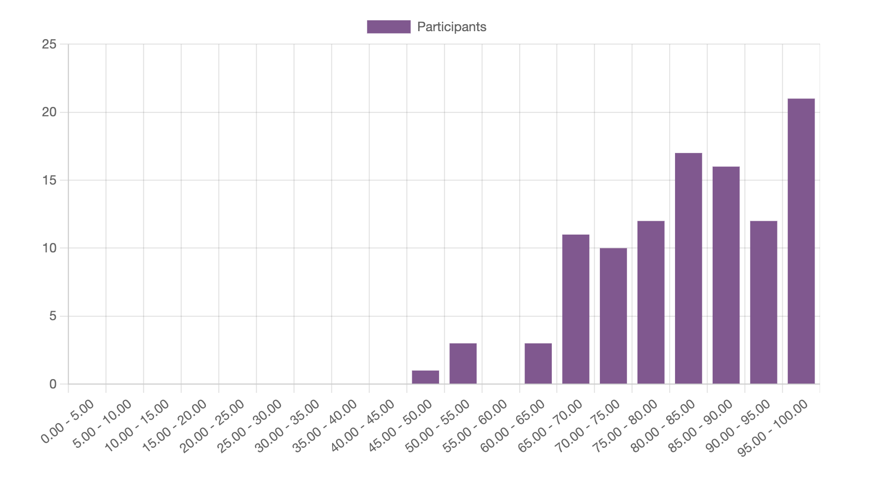
_images/EMET7001quiz2.png — Fig. 23 Distribution of results for Online test 2#

Teaching break: next two weeks April 1st to 14th

No teaching
No tutorials
Next lecture is on April 16th
Next online test is on April 22nd, after the next lecture

Have a good break!

📖 Univariate differentiation#

⏱ | words

Sources and reading guide#

Limit for functions#

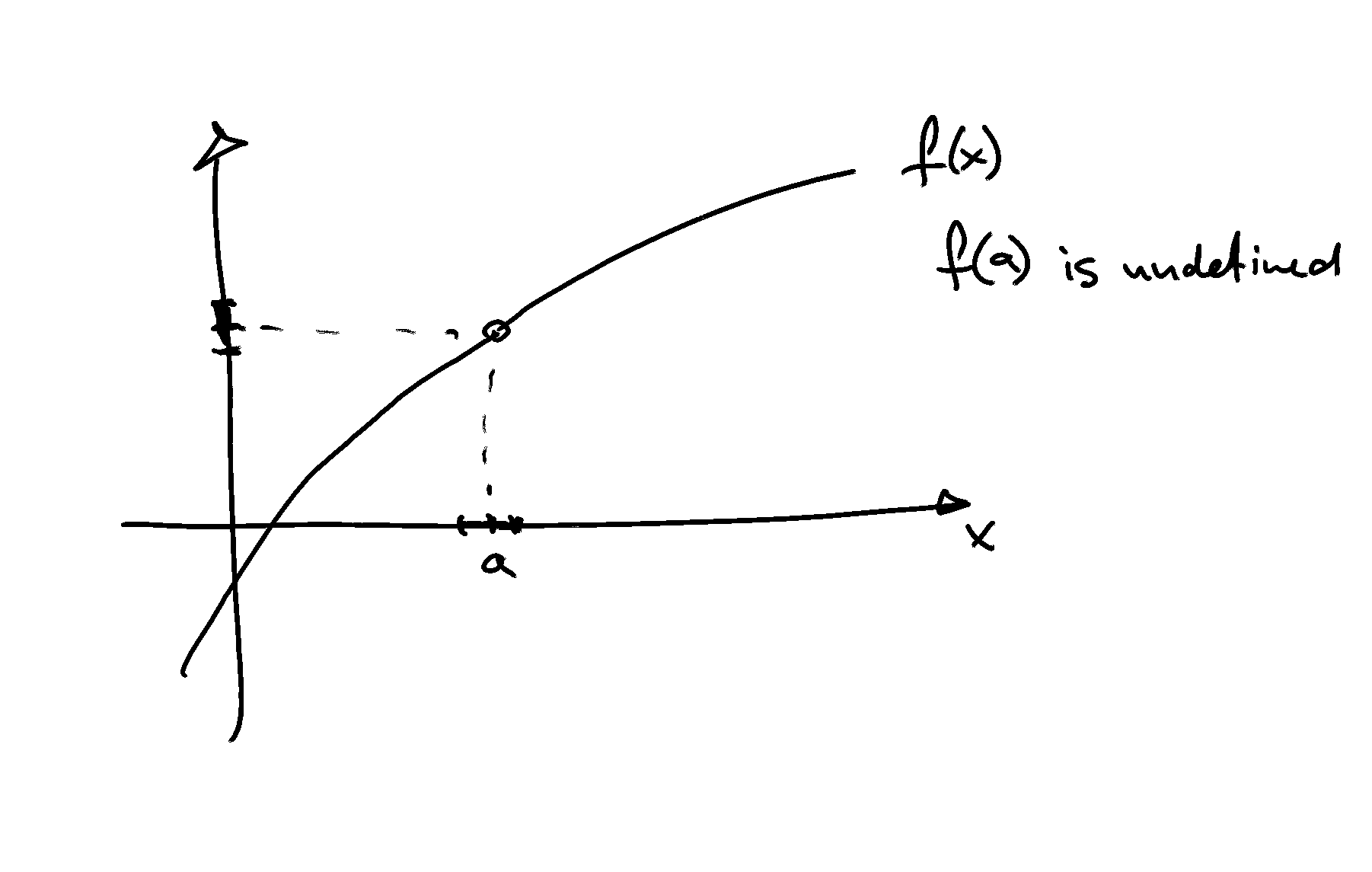
Consider a univariate function $f: \mathbb{R} \rightarrow \mathbb{R}$ written as $f(x)$

The domain of $f$ is $\mathbb{R}$, the range of $f$ is a (possibly improper) subset of $\mathbb{R}$

[Spivak, 2006] (p. 90) provides the following informal definition of a limit: “The function $f$ approaches the limit $l$ near [the point $x =$] $a$, if we can make $f(x)$ as close as we like to $l$ by requiring that $x$ be sufficiently close to, but unequal to, $a$.”

Definition

The function $f: \mathbb{R} \rightarrow \mathbb{R}$ approaches the limit $l$ near [the point $x = a$] if for every $\epsilon > 0$, there is some $\delta > 0$ such that, for all $x$ such as $0 < |x − a| < \delta$, $|f(x) − l | < \epsilon$.

The absolute value $|\cdot|$ in this definition plays the role of general distance function $\|\cdot\|$ which would be appropriate for the functions from $\mathbb{R}^n$ to $\mathbb{R}^k$. We will also use $d(x,a)$ to denote distance, i.e. $d(x,a) = |x-a|$.

Suppose that the limit of $f$ as $x$ approaches $a$ is $l$. We can write this as

\[ \lim_{x \rightarrow a} f(x) = l \]

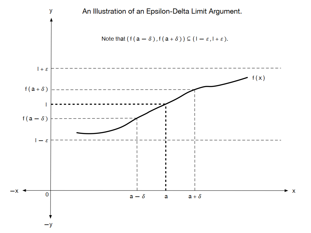
_images/epsilon_delta.png — Fig. 24 An illustration of an epsilon-delta limit argument#

The structure of $\epsilon–\delta$ arguments#

Suppose that we want to attempt to show that $\lim _{x \rightarrow a} f(x)=b$.

In order to do this, we need to show that, for any choice $\epsilon>0$, there exists some $\delta_{\epsilon}>0$ such that, whenever $|x-a|<\delta_{\epsilon}$, it is the case that $|f(x)-b|<\epsilon$.

We write $\delta_{\epsilon}$ to indicate that the choice of $\delta$ is allowed to vary with the choice of $\epsilon$.

An often fruitful approach to the construction of a formal $\epsilon$-$\delta$ limit argument is to proceed as follows:

Start with the end-point that we need to establish: $|f(x)-b|<\epsilon$.
Use appropriate algebraic rules to rearrange this “final” inequality into something of the form $|k(x)(x-a)|<\epsilon$.
This new version of the required inequality can be rewritten as $|k(x)||(x-a)|<\epsilon$.
If $k(x)=k$, a constant that does not vary with $x$, then this inequality becomes $|k||x-a|<\epsilon$. In such cases, we must have $|x-a|<\frac{\epsilon}{|k|}$, so that an appropriate choice of $\delta_{\epsilon}$ is $\delta_{\epsilon}=\frac{\epsilon}{|k|}$.
If $k(x)$ does vary with $x$, then we have to work a little bit harder.

Suppose that $k(x)$ does vary with $x$. How might we proceed in that case? One possibility is to see if we can find a restriction on the range of values for $\delta$ that we consider that will allow us to place an upper bound on the value taken by $|k(x)|$.

In other words, we try and find some restriction on $\delta$ that will ensure that $|k(x)|<K$ for some finite $K>0$. The type of restriction on the values of $\delta$ that you choose would ideally look something like $\delta<D$, for some fixed real number $D>0$. (The reason for this is that it is typically small deviations of $x$ from a that will cause us problems rather than large deviations of $x$ from a.)

If $0<|k(x)|<K$ whenever $0<\delta<D$, then we have

\[ |k(x)||x-a|<\epsilon \Longleftarrow K|x-a|<\epsilon \Longleftrightarrow|x-a|<\frac{\epsilon}{K} . \]

In such cases, an appropriate choice of $\delta_{\epsilon}$ is $\delta_{\epsilon}=\min \left\{\frac{\epsilon}{K}, D\right\}$.

Heine and Cauchy definitions of the limit for functions#

As a side note, let’s mention that there are two ways to define the limit of a function $f$.

The above $\epsilon$-$\delta$ definition is is due to Augustin-Louis Cauchy.

The limit for functions can also be defined through the limit of sequences we were talking about in the last lecture. This equivalent definition is due to Eduard Heine

Definition (Limit of a function due to Heine)

Given the function $f: A \subset \mathbb{R} \to \mathbb{R}$, $a \in \mathbb{R}$ is a limit of $f(x)$ as $x \to x_0 \in A$ if

\[\forall \{x_n\} \in A \colon \lim_{n \to \infty} x_n = x_0 \in A \quad \implies \quad f(x_n) \to a \]

note the crucial requirement that $f(x_n) \to a$ has to hold for all converging to $x_0$ sequences $\{x_n\}$ in $A$
note also how the Cauchy definition is similar to the definition of a limit to a sequence

Fact

Cauchy and Heine definitions of the function limit are equivalent

Therefore we can use the same notation of the definition of the limit of a function

\[\lim_{x \to x_0} f(x) = a \quad \text{or} \quad f(x) \to a \; \text{as} \; x \to x_0\]

Some useful rules about limits#

In practice, we would like to be able to find at least some limits without having to resort to the formal “epsilon-delta” arguments that define them. The following rules can sometimes assist us with this.

Fact

Let $c \in \mathbb{R}$ be a fixed constant, $a \in \mathbb{R}, \alpha \in \mathbb{R}, \beta \in \mathbb{R}, n \in \mathbb{N}$, $f: \mathbb{R} \longrightarrow \mathbb{R}$ be a function for which $\lim _{x \rightarrow a} f(x)=\alpha$, and $g: \mathbb{R} \longrightarrow \mathbb{R}$ be a function for which $\lim _{x \rightarrow a} g(x)=\beta$. The following rules apply for limits:

$\lim _{x \rightarrow a} c=c$ for any $a \in \mathbb{R}$.
$\lim _{x \rightarrow a}(c f(x))=c\left(\lim _{x \rightarrow a} f(x)\right)=c \alpha$.
$\lim _{x \rightarrow a}(f(x)+g(x))=\left(\lim _{x \rightarrow a} f(x)\right)+\left(\lim _{x \rightarrow a} g(x)\right)=\alpha+\beta$.
$\lim _{x \rightarrow a}(f(x) g(x))=\left(\lim _{x \rightarrow a} f(x)\right)\left(\lim _{x \rightarrow a} g(x)\right)=\alpha \beta$.
$\lim _{x \rightarrow a}\left(\frac{f(x)}{g(x)}\right)=\frac{\lim _{x \rightarrow a} f(x)}{\lim _{x \rightarrow a} g(x)}=\frac{\alpha}{\beta}$ whenever $\beta \neq 0$.
$\lim _{x \rightarrow a} \sqrt[n]{f(x)}=\sqrt[n]{\lim _{x \rightarrow a} f(x)}=\sqrt[n]{\alpha}$ whenever $\sqrt[n]{\alpha}$ is defined.
$\lim _{x \rightarrow a} \ln f(x)=\ln \lim _{x \rightarrow a} f(x)=\ln \alpha$ whenever $\ln \alpha$ is defined.
$\lim _{x \rightarrow a} e^{f(x)}=\exp\big(\lim _{x \rightarrow a} f(x)\big)=e^{\alpha}$
After we have learned about differentiation, we will learn about another useful rule for limits that is known as “L’Hopital’s rule”.

Example

This is an example in which the chosen function will be very nicely behaved at all points $x \in \mathbb{R}$.
Consider the function $f(x)=x$ and the point $x=2$. We will show formally that $\lim _{x \rightarrow 2} f(x)=2$.
Note that

\[ d(f(x), 2)=|x-2|=d(x, 2) . \]

Let $\epsilon>0$. We have

\[ d(f(x), 2)<\epsilon \Longleftrightarrow|x-2|<\epsilon \]

Suppose that we let $\delta_{\epsilon}=\epsilon$. Since $\epsilon>0$, we must have $\delta_{\epsilon}>0$.
Consider points in $\mathbb{R}$ that satisfy the condition

\[ 0<d(x, 2)<\delta_{\epsilon} \]

Consider points in $\mathbb{R}$ that satisfy the condition

\[ 0<d(x, 2)<\delta_{\epsilon} \]

Note that

\[\begin{split} \begin{aligned} 0<d(x, 2)<\delta_{\epsilon} & \Longleftrightarrow 0<|x-2|<\delta_{\epsilon} \\ & \Longleftrightarrow 0<d(f(x), 2)<\delta_{\epsilon} \end{aligned} \end{split}\]

Thus we have

\[ 0<d(x, 2)<\delta_{\epsilon} \Longrightarrow d(f(x), 2)<\delta_{\epsilon} \text {. } \]

Since we chose $\epsilon>0$ arbitrarily, this must be true for all $\epsilon>0$. This means that $\lim _{x \rightarrow 2} f(x)=2$.

Example

This example is drawn from Willis Lauritz Peterson of the University of Utah.
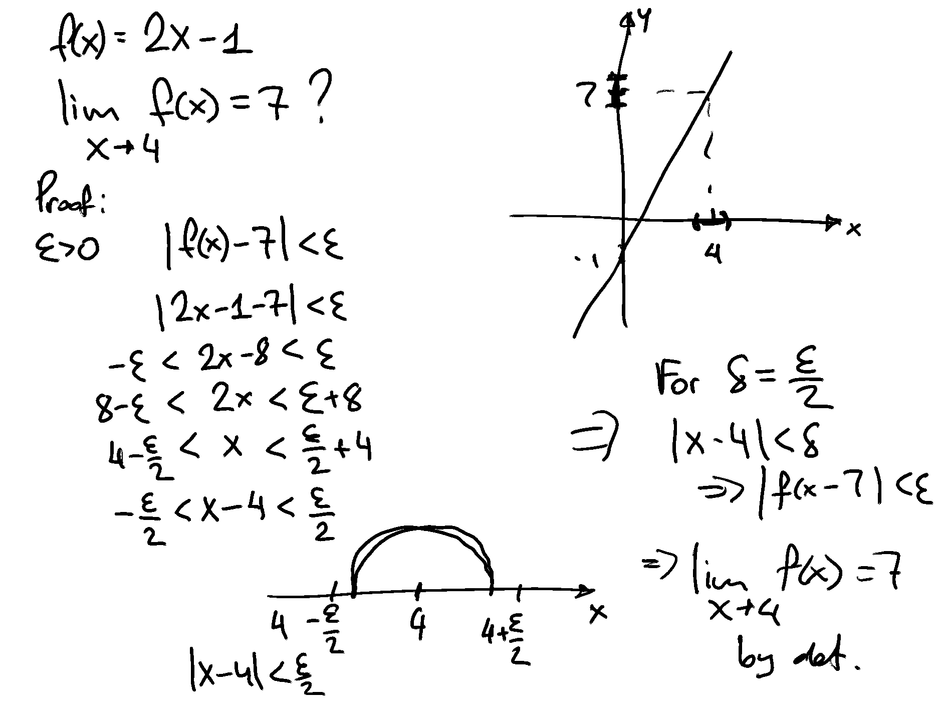
Consider the mapping $f: \mathbb{R} \longrightarrow \mathbb{R}$ defined by $f(x)=7 x-4$. We want to show that $\lim _{x \rightarrow 2} f(x)=10$.
Note that $|f(x)-10|=|7 x-4-10|=|7 x-14|=|7(x-2)|=$ $|7||x-2|=7|x-2|$.
We require $|f(x)-10|<\epsilon$. Note that

\[ |f(x)-10|<\epsilon \Longleftrightarrow 7|x-2|<\epsilon \Longleftrightarrow|x-2|<\frac{\epsilon}{7} \]

Thus, for any $\epsilon>0$, if $\delta_{\epsilon}=\frac{\epsilon}{7}$, then $|f(x)-10|<\epsilon$ whenever $|x-2|<\delta_{\epsilon}$.

Example

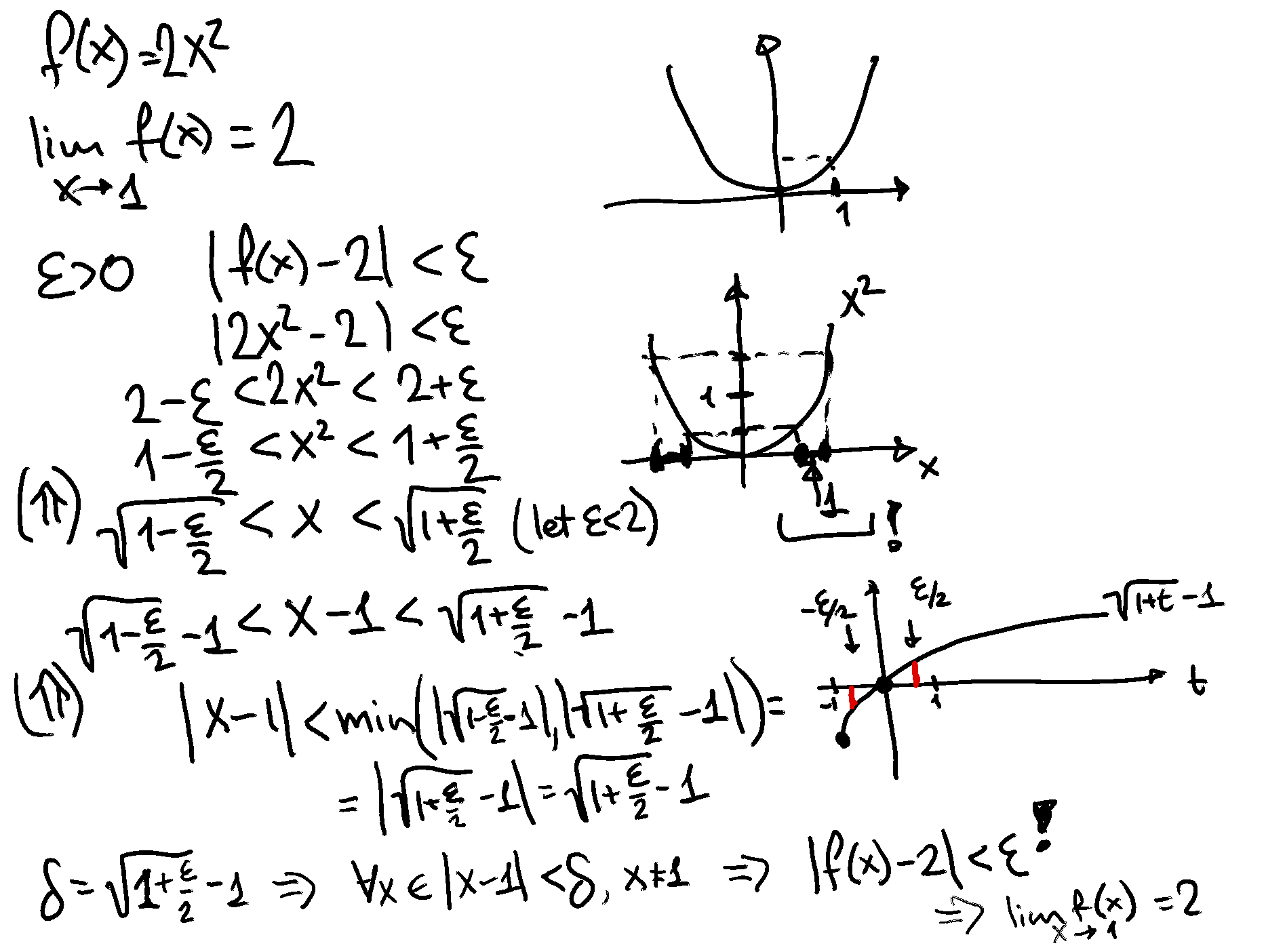
Consider the mapping $f: \mathbb{R} \longrightarrow \mathbb{R}$ defined by $f(x)=x^{2}$. We want to show that $\lim _{x \rightarrow 2} f(x)=4$.
Note that $|f(x)-4|=\left|x^{2}-4\right|=|(x+2)(x-2)|=|x+2||x-2|$.
Suppose that $|x-2|<\delta$, which in turn means that $(2-\delta)<x<(2+\delta)$. Thus we have $(4-\delta)<(x+2)<(4+\delta)$.
Let us restrict attention to $\delta \in(0,1)$. This gives us $3<(x+2)<5$, so that $|x+2|<5$.
Thus, when $|x-2|<\delta$ and $\delta \in(0,1)$, we have $|f(x)-4|=|x+2||x-2|<5 \delta$.
We require $|f(x)-4|<\epsilon$. One way to ensure this is to set $\delta_{\epsilon}=\min \left(1, \frac{\epsilon}{5}\right)$.

Example

This example is drawn from Willis Lauritz Peterson of the University of Utah.

Consider the mapping $f: \mathbb{R} \rightarrow \mathbb{R}$ defined by $f(x) = x^2 − 3x + 1$.

We want to show that $lim_{x \rightarrow 2} f(x ) = −1$.

Note that $|f(x) − (−1)| = |x^2 − 3x + 1 + 1| = |x^2 − 3x + 2| = |(x − 1)(x − 2)| = |x − 1||x − 2|$.
Suppose that $|x − 2| < \delta$, which in turn means that $(2 − \delta) < x < (2 + \delta)$. Thus we have $(1 − \delta) < (x − 1) < (1 + \delta)$.
Let us restrict attention to $\delta \in (0, 1)$. This gives us $0 < (x − 1) < 2$, so that $|x − 1| < 2$.
Thus, when $|x − 2| < \delta$ and $\delta \in (0, 1)$, we have $|f(x) − (−1)| = |x − 1||x − 2| < 2\delta$.
We require $|f(x) − (−1)| < \epsilon$. One way to ensure this is to set $\delta_\epsilon = \min(1, \frac{\epsilon}{2} )$.

Example

Limits can sometimes exist even when the function being considered is not so well behaved. One such example is provided by [Spivak, 2006] (pp. 91–92). It involves the use of a trigonometric function.

The example involves the function $f: \mathbb{R} \setminus 0 \rightarrow \mathbb{R}$ that is defined by $f(x) = x sin ( \frac{1}{x})$.

Clearly this function is not defined when $x = 0$. Furthermore, it can be shown that $\lim_{x \rightarrow 0} sin ( \frac{1}{x})$ does not exist. However, it can also be shown that $lim_{x \rightarrow 0} f(x) = 0$.

The reason for this is that $sin (\theta) \in [−1, 1]$ for all $\theta \in \mathbb{R}$. Thus $sin ( \frac{1}{x} )$ is bounded above and below by finite numbers as $x \rightarrow 0$. This allows the $x$ component of $x sin (\frac{1}{x})$ to dominate as $x \rightarrow 0$.

Example

Limits do not always exist. In this example, we consider a case in which the limit of a function as $x$ approaches a particular point does not exist.

Consider the mapping $f: \mathbb{R} \rightarrow \mathbb{R}$ defined by

\[\begin{split} f(x ) = \begin{cases} 1 \quad \text{ if } x > 5; \\ 0 \quad \text{ if } x < 5 \end{cases} \end{split}\]

We want to show that $\lim_{x \rightarrow 5} f(x)$ does not exist.

Suppose that the limit does exist. Denote the limit by $l$. Recall that $d (x, y ) = \{ (y − x )2 \}^{\frac{1}{2}} = |y − x |$. Let $\delta > 0$.

If $|5 − x | < \delta$, then $5 − \delta < x < 5 + \delta$, so that $x \in (5 − \delta, 5 + \delta)$.

Note that $x \in (5 − \delta, 5 + \delta) = (5 − \delta, 5) \cup [5, 5 + \delta)$, where $(5 − \delta, 5) \ne \varnothing$ and $[5, 5 + \delta) \ne \varnothing$.

Thus we know the following:

There exist some $x \in (5 − \delta, 5) \subseteq (5 − \delta, 5 + \delta)$, so that $f(x) = 0$ for some $x \in (5 − \delta, 5 + \delta)$.
There exist some $x \in [5, 5 + \delta) \subseteq (5 − \delta, 5 + \delta)$, so that $f(x) = 1$ for some $x \in (5 − \delta, 5 + \delta)$.
The image set under $f$ for $(5 − \delta, 5 + \delta)$ is $f ((5 − \delta, 5 + \delta)) = \{ f(x) : x \in (5 − \delta, 5 + \delta) \} = \{ 0, 1 \} \subseteq [0, 1]$.
Note that for any choice of $\delta > 0$, $[0, 1]$ is the smallest connected interval that contains the image set $f ((5 − \delta, 5 + \delta)) = \{ 0, 1 \}$.

Hence, in order for the limit to exist, we need $[0, 1] \subseteq (l − \epsilon, l + \epsilon)$ for all $\epsilon > 0$. But for $\epsilon \in (0, \frac{1}{2})$, there is no $l \in \mathbb{R}$ for which this is the case. Thus we can conclude that $\lim_{x \rightarrow 5} f(x)$ does not exist.

Continuity#

Our focus here is on continuous real-valued functions of a single real variable. In other words, functions of the form $f : X \rightarrow \mathbb{R}$ where $X \subseteq \mathbb{R}$.

Before looking at the picky technical details of the concept of continuity, it is worth thinking about that concept intuitively. Basically, a real-valued function of a single real-valued variable is continuous if you could potentially draw its graph without lifting your pen from the page. In other words, there are no holes in the graph of the function and there are no jumps in the graph of the function.

Definition

Let $f \colon A \to \mathbb{R}$

$f$ is called continuous at $a \in A$ if

\[\forall \{x_n\} \in A \colon \lim_{n \to \infty} x_n = a \in A \quad \implies \quad f(x_n) \to f(a) \]

Or, alternatively,

\[\lim_{x \to a} f(x) = f(a)\]

Definition

$f: A \to \mathbb{R}$ is called continuous if it is continuous at every $x \in A$

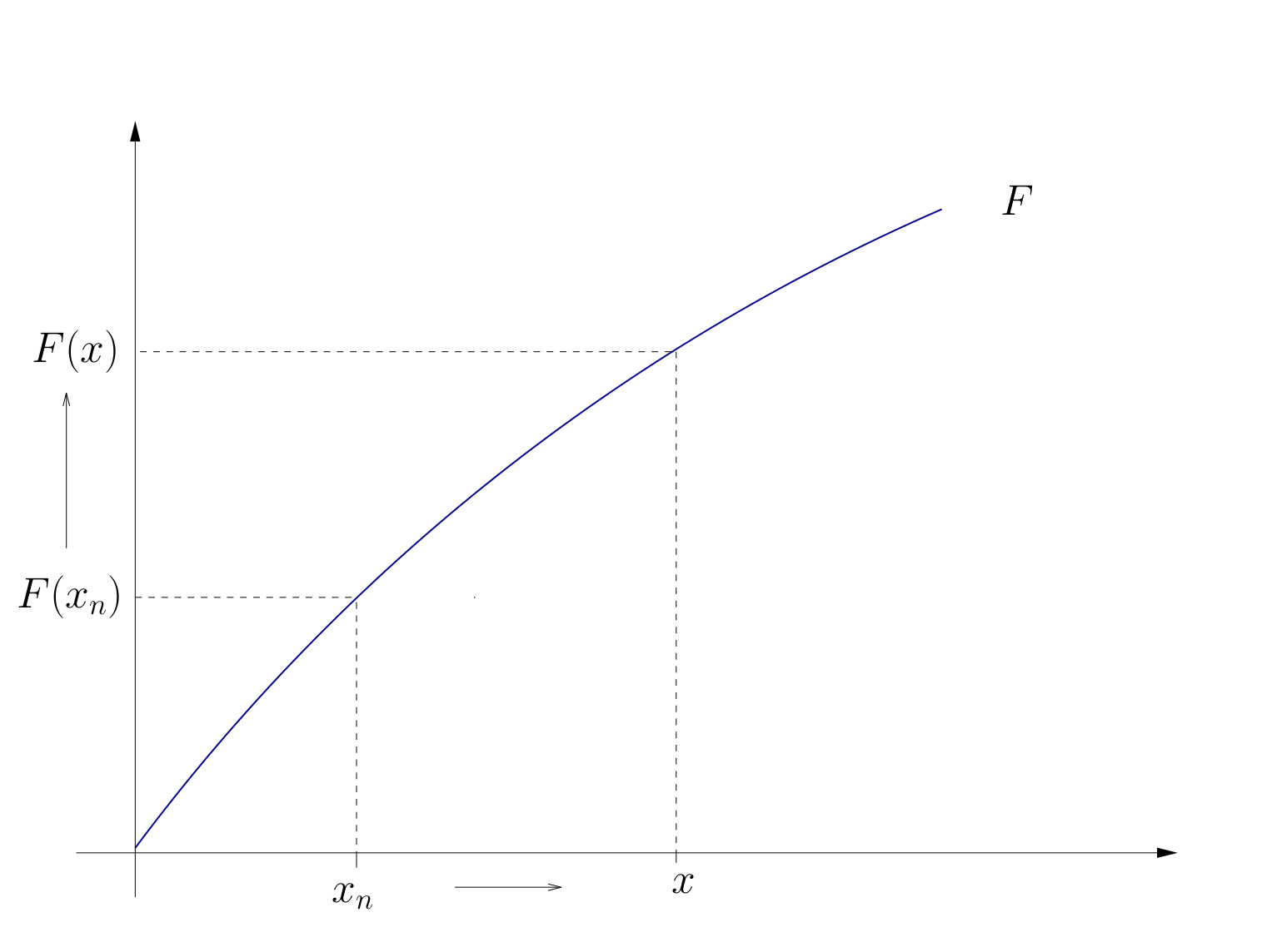
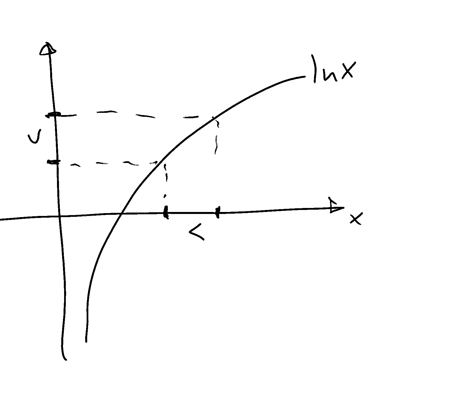
_images/cont_func.png — Fig. 25 Continuous function#

Example

Function $f(x) = \exp(x)$ is continuous at $x=0$

Proof:

Consider any sequence $\{x_n\}$ which converges to $0$

We want to show that for any $\epsilon>0$ there exists $N$ such that $n \geq N \implies |f(x_n) - f(0)| < \epsilon$. We have

\[\begin{split}\begin{array}{l} |f(x_n) - f(0)| = |\exp(x_n) - 1| < \epsilon \quad \iff \\ \exp(x_n) - 1 < \epsilon \; \text{ and } \; \exp(x_n) - 1 > -\epsilon \quad \iff \\ x_n < \ln(1+\epsilon) \; \text{ and } \; x_n > \ln(1-\epsilon) \quad \Longleftarrow \\ | x_n - 0 | < \min \big(\ln(1+\epsilon),\ln(1-\epsilon) \big) = \ln(1-\epsilon) \end{array}\end{split}\]

Because due to $x_n \to x$ for any $\epsilon' = \ln(1-\epsilon)$ there exists $N$ such that $n \geq N \implies |x_n - 0| < \epsilon'$, we have $f(x_n) \to f(x)$ by definition. Thus, $f$ is continuous at $x=0$.

Fact

Some functions known to be continuous on their domains:

$f: x \mapsto x^\alpha$
$f: x \mapsto |x|$
$f: x \mapsto \log(x)$
$f: x \mapsto \exp(x)$
$f: x \mapsto \sin(x)$
$f: x \mapsto \cos(x)$

Types of discontinuities#

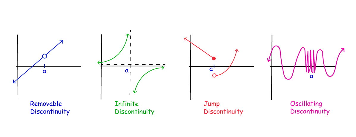
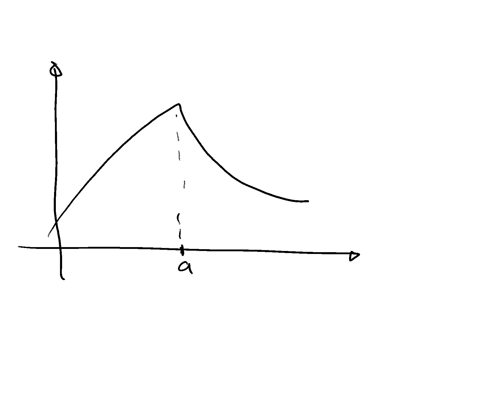
_images/4-types-of-discontinuity.png — Fig. 26 4 common types of discontinuity#

Example

The indicator function $x \mapsto \mathbb{1}\{x > 0\}$ has a jump discontinuity at $0$.

Fact

Let $f$ and $g$ be functions and let $\alpha \in \mathbb{R}$

If $f$ and $g$ are continuous at $x$ then so is $f + g$, where

\[(f + g)(x) := f(x) + g(x)\]

If $f$ is continuous at $x$ then so is $\alpha f$, where

\[(\alpha f)(x) := \alpha f(x)\]

If $f$ and $g$ are continuous at $x$ and real valued then so is $f \circ g$, where

\[(f \circ g)(x) := f( g(x))\]

In the latter case, if in addition $g(x) \ne 0$, then $f/g$ is also continuous.

Proof

Just repeatedly apply the properties of the limits

Let’s just check that

\[\text{$f$ and $g$ continuous at $x$} \implies \text{$f + g$ continuous at $x$}\]

Let $f$ and $g$ be continuous at $x$

Pick any $x_n \to x$

We claim that $f(x_n) + g(x_n) \to f(x) + g(x)$

By assumption, $f(x_n) \to f(x)$ and $g(x_n) \to g(x)$

From this and the triangle inequality we get

\[\| f(x_n) + g(x_n) - (f(x) + g(x)) \| \leq \]

\[\leq \| f(x_n) - f(x) \| + \| g(x_n) - g(x) \| \to 0\]

As a result, set of continuous functions is “closed” under elementary arithmetic operations

Example

The function $f \colon \mathbb{R} \to \mathbb{R}$ defined by

\[f(x) = \frac{\exp(x) + \sin(x)}{2 + \cos(x)} + \frac{x^4}{2} - \frac{\cos^3(x)}{8!}\]

is continuous (we just have to be careful to ensure that denominator is not zero – which it is not for all $x\in\mathbb{R}$)

Example

An example of oscillating discontinuity is the function $f(x) = \sin(1/x)$ which is discontinuous at $x=0$.

Video to illustrate this function

Example

Consider the mapping $f : \mathbb{R} \rightarrow \mathbb{R}$ defined by $f(x ) = x_2$. We want to show that $f(x)$ is continuous at the point $x = 2$.

Recall that $d (x, y ) = \{ (y − x )2 \}^{\frac{1}{2}} = |y − x |$.

Note that $|f (2) − f(x)| = |f(x) − f (2)| = |x^2 − 4| = |x − 2||x + 2|$.

Suppose that $|2 − x | < \delta$. This means that $|x − 2| < \delta$, which in turn means that $(2 − \delta) < x < (2 + \delta)$. Thus we have $(4 − \delta) < (x + 2) < (4 + \delta)$.

Let us restrict attention to $\delta \in (0, 1)$. This gives us $3 < (x + 2) < 5$, so that $|x + 2| < 5$.

We have $|f (2) − f(x)| = |f(x) − f (2)| = |x − 2||x + 2| < (\delta)(5) = 5\delta$.

We require $|f (2) − f(x)| < \epsilon$. One way to ensure this is to set $\delta = min(1, \frac{\epsilon}{5})$.

Example

Consider the mapping $f: \mathbb{R} \rightarrow \mathbb{R}$ defined by $f(x ) = x$. We want to show that $f(x)$ is continuous for all $x \in X$.

Recall that $d (x, y ) = \{ (y − x )2 \}^{\frac{1}{2}} = |y − x |$.

Consider an arbitrary point $x = a$. Note that $|f (a) − f(x)| = |a − x |$.

Suppose that $|a − x | < \delta$.

Note that if we set $\delta = \epsilon$, we have $|f (a) − f(x)| < \epsilon$.

Thus we know that $f$ is continuous at the point $x = a$. Since $a$ was chosen arbitrarily, we now that this is true for all $a \in \mathbb{R}$. This means that $f$ is continuous for all $x \in \mathbb{R}$.

Example

Consider the mapping $f: \mathbb{R} \rightarrow \mathbb{R}$ defined by

\[\begin{split} f(x ) = \begin{cases} 1 \quad \text{ if } x > 5; \\ 0 \quad \text{ if } x < 5 \end{cases} \end{split}\]

We have already shown that $\lim_{x \rightarrow 5} f(x)$ does not exist. This means that it is impossible for $lim_{x \rightarrow 5} f(x) = f (5)$. As such, we know that $f(x)$ is not continuous at the point $x = 5$.

This means that f(x) is not a continuous function.

However, it can be shown that (i) $f(x )$ is continuous on the interval $(−\infty, 5)$, and that (ii) $f(x)$ is continuous on the interval $(5, \infty)$. Can you explain why this is the case?

Example

Consider the mapping $f: \mathbb{R} \rightarrow \mathbb{R}$ defined by

\[\begin{split} f(x) = \begin{cases} \frac{1}{x} \quad \text{ if } x \ne 0; \\ 0 \quad \text{ if } x = 0. \end{cases} \end{split}\]

This function is a rectangular hyperbola when $x \ne 0$, but it takes on the value $0$ when $x = 0$. Recall that the rectangular hyperbola part of this function is not defined at the point $x = 0$.

This function is discontinuous at the point $x = 0$. Illustrate the graph of this function on the whiteboard.

Example

Consider the mapping $f: \mathbb{R} \rightarrow \mathbb{R}$ defined by

\[\begin{split} f(x) = \begin{cases} 1 \quad \text{ if } x \in Q; \\ 0 \quad \text{ if } x \notin Q \end{cases} \end{split}\]

This function is sometimes known as Dirichlet’s discontinuous function. It is discontinuous at every point in its domain.

Derivatives#

If it exists, the derivative of a function tells us the direction and magnitude of the change in the dependent variable that will be induced by a very small increase in the independent variable.

If it exists, the derivative of a function at a point is equal to the slope of the straight line that is tangent to the function at that point.

You should try and guess now what the derivative of a linear function of the form $f(x) = ax + b$ will be.

Definition#

Consider a function $f : X \rightarrow \mathbb{R}$, where $X \subseteq \mathbb{R}$. Let $(x_0, f (x_0))$ and $(x_0 + h, f (x_0 + h))$ be two points that lie on the graph of this function.

Draw a straight line between these two points. The slope of this line is

\[\begin{split} \begin{align*} \frac{\text{rise}}{\text{run}} &= \frac{y_2 − y_1}{x_2 − x_1} \\ &= \frac{f (x_0 + h) − f (x_0)}{x_0 + h − x_0} \\ &= \frac{f (x_0 + h) − f (x_0)}{h} \end{align*} \end{split}\]

What happens to this slope as $h \rightarrow 0$ (that is, as the second point gets very close to the first point?

Definition

The (first) derivative of the function $f(x)$ at the point $x=x_{0}$, if it exists, is defined to be

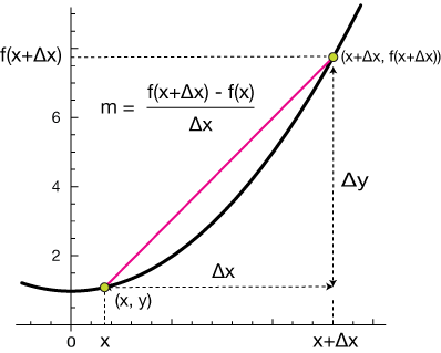
\[ f^{\prime}\left(x_{0}\right) =\frac{d f}{d x}(x_{0}) =\lim _{h \rightarrow 0} \frac{f\left(x_{0}+h\right)-f\left(x_{0}\right)}{h} . \]

This is simply the slope of the straight line that is tangent to the function $f(x)$ at the point $x=x_{0}$.

We will now proceed to use this definition to find the derivative of some simple functions. This is sometimes called “finding the derivative of a function from first principles”.

Example: the derivative of a constant function

Consider the function $f: X \longrightarrow \mathbb{R}$ defined by $f(x)=b$, where $b \in \mathbb{R}$ is a constant. Clearly we have $f\left(x_{0}\right)=f\left(x_{0}+h\right)=b$ for all choices of $x_{0}$ and $h$.

Thus we have

\[ \frac{f\left(x_{0}+h\right)-f\left(x_{0}\right)}{h}=\frac{b-b}{h}=\frac{0}{h}=0 \]

for all choices of $x_{0}$ and $h$.

This means that

\[ \lim _{h \rightarrow 0} \frac{f\left(x_{0}+h\right)-f\left(x_{0}\right)}{h}=\lim _{h \rightarrow 0} 0=0 \]

As such, we can conclude that

\[ f^{\prime}(x)=\frac{d f}{d x}=0 \]

Example: the derivative of a linear function

Consider the function $f: X \longrightarrow \mathbb{R}$ defined by $f(x)=a x+b$. Note that

\[\begin{split} \begin{aligned} f(x+h) & =a(x+h)+b \\ & =a x+a h+b \\ & =a x+b+a h \\ & =f(x)+a h . \end{aligned} \end{split}\]

Thus we have

\[ \frac{f(x+h)-f(x)}{h}=\frac{f(x)+a h-f(x)}{h}=\frac{a h}{h}=a . \]

This means that $\lim _{h \rightarrow 0} \frac{f\left(x_{0}+h\right)-f\left(x_{0}\right)}{h}=\lim _{h \rightarrow 0} a=a$.

As such, we can conclude that $f^{\prime}(x)=\frac{d f}{d x}=a$.

Example: the derivative of a quadratic power function

Consider the function $f: X \longrightarrow \mathbb{R}$ defined by $f(x)=x^{2}$. Note that

\[\begin{split} \begin{aligned} f(x+h) & =(x+h)^{2} \\ & =x^{2}+2 x h+h^{2} \\ & =f(x)+2 x h+h^{2} \end{aligned} \end{split}\]

Thus we have

\[\begin{split} \begin{aligned} \frac{f(x+h)-f(x)}{h} & =\frac{f(x)+2 x h+h^{2}-f(x)}{h} \\ & =\frac{2 x h+h^{2}}{h} \\ & =2 x+h . \end{aligned} \end{split}\]

This means that $\lim _{h \rightarrow 0} \frac{f\left(x_{0}+h\right)-f\left(x_{0}\right)}{h}=\lim _{h \rightarrow 0}(2 x+h)=2 x$.

As such, we can conclude that $f^{\prime}(x)=\frac{d f}{d x}=2 x$

Example: the derivative of a quadratic polynomial function

Consider the function $f: X \longrightarrow \mathbb{R}$ defined by $f(x)=a x^{2}+b x+c$. Note that

\[\begin{split} \begin{aligned} f(x+h) & =a(x+h)^{2}+b(x+h)+c \\ & =a\left(x^{2}+2 x h+h^{2}\right)+b x+b h+c \\ & =a x^{2}+2 a x h+a h^{2}+b x+b h+c \\ & =\left(a x^{2}+b x+c\right)+(2 a x+b) h+a h^{2} \\ & =f(x)+(2 a x+b) h+a h^{2} . \end{aligned} \end{split}\]

Thus we have

\[\begin{split} \begin{aligned} \frac{f(x+h)-f(x)}{h} & =\frac{f(x)+(2 a x+b) h+a h^{2}-f(x)}{h} \\ & =\frac{(2 a x+b) h+a h^{2}}{h} \\ & =(2 a x+b)+a h \\ & =2 a x+b+a h . \end{aligned} \end{split}\]

This means that

\[ \lim _{h \rightarrow 0} \frac{f\left(x_{0}+h\right)-f\left(x_{0}\right)}{h}=\lim _{h \rightarrow 0}(2 a x+b+a h)=2 a x+b \]

As such, we can conclude that $f^{\prime}(x)=\frac{d f}{d x}=2 a x+b$.

Fact (Binomial theorem)

The binomial theorem

Suppose that $x, y \in \mathbb{R}$ and $n \in \mathbb{Z}_+ = \mathbb{N} \cup \{0\}$.

We have

\[ (x + y)^n = \sum_{k = 0}^{n} \binom{n}{k} x^{(n−k)} y^k \]

where $\binom{n}{k} = C_{n,k} = \frac{n!}{k! (n − k)!}$ is known as a binomial coefficient (read “$n$ choose $k$” because this is the number of ways to choose a subset of $k$ elements from a set of $n$ elements). $n! = \prod_{k=1}^n k$ denotes a factorial of $n$, and $0! = 1$ by definition.

Useful property is $\binom{n}{k} = C_{n,k} = C_{n-1,k-1}+C_{n-1,k}$ is illustrated by Pascal’s triangle.

Example: the derivative of a positive integer power function

Consider the function $f: \mathbb{R} \longrightarrow \mathbb{R}$ defined by $f(x)=x^{n}$, where $n \in \mathbb{N}=\mathbb{Z}_{++}$. We know from the binomial theorem that

\[\begin{split} \begin{aligned} f(x+h) & =(x+h)^{n} \\ & =\sum_{r=0}^{n}\left(\begin{array}{l} n \\ r \end{array}\right) x^{n-r} h^{r} \\ & =\left(\begin{array}{l} n \\ 0 \end{array}\right) x^{n} h^{0}+\sum_{r=1}^{n}\left(\begin{array}{l} n \\ r \end{array}\right) x^{n-r} h^{r} \\ & =1 x^{n}(1)+\sum_{r=1}^{n}\left(\begin{array}{l} n \\ r \end{array}\right) x^{n-r} h^{r} \\ & =x^{n}+\sum_{r=1}^{n}\left(\begin{array}{l} n \\ r \end{array}\right) x^{n-r} h^{r} . \end{aligned} \end{split}\]

Thus we have

\[\begin{split} \begin{aligned} \frac{f(x+h)-f(x)}{h} & =\frac{f(x)+\sum_{r=1}^{n}\left(\begin{array}{l} n \\ r \end{array}\right) x^{n-r} h^{r}-f(x)}{h} \\ & =\frac{\sum_{r=1}^{n}\left(\begin{array}{l} n \\ r \end{array}\right) x^{n-r} h^{r}}{h} \\ & =\sum_{r=1}^{n}\left(\begin{array}{l} n \\ r \end{array}\right) x^{n-r} h^{r-1} \\ & =\left(\begin{array}{l} n \\ 1 \end{array}\right) x^{n-1} h^{0}+\sum_{r=2}^{n}\left(\begin{array}{l} n \\ r \end{array}\right) x^{n-r} h^{r-1} \\ & =n x^{n-1}(1)+\sum_{r=2}^{n}\left(\begin{array}{l} n \\ r \end{array}\right) x^{n-r} h^{r-1} \end{aligned} \end{split}\]

\[\begin{split} \frac{f(x+h)-f(x)}{h} & =n x^{n-1}+\sum_{r=2}^{n}\left(\begin{array}{l} n \\ r \end{array}\right) x^{n-r} h^{r-1} \end{split}\]

This means that

\[\begin{split} \lim _{h \rightarrow 0} \frac{f\left(x_{0}+h\right)-f\left(x_{0}\right)}{h}=\lim _{h \rightarrow 0}\left(n x^{n-1}+\sum_{r=2}^{n}\left(\begin{array}{l} n \\ r \end{array}\right) x^{n-r} h^{r-1}\right)=n x^{n-1} \end{split}\]

As such, we can conclude that

\[ f^{\prime}(x)=\frac{d f}{d x}=n x^{n-1} \]

Example: derivative of an $e^x$

Consider the function $f: \mathbb{R} \longrightarrow \mathbb{R}_{++}$ defined by $f(x)=e^x$, where $e$ in Euler’s constant. Recall that by definition $e = \lim_{n \to \infty} (1+\frac{1}{n})^n$

\[ \lim_{h \to 0} \frac{f(x+h)-f(x)}{h} =\lim_{h \to 0} \frac{e^{x+h}-e^x}{h} =\lim_{h \to 0} \frac{e^x(e^h-1)}{h} \]

Consider $\lim_{h \to 0}\frac{e^h-1}{h}$ after substitution $t=(e^h-1)^{-1}$ $\Leftrightarrow$ $h = \ln(t^{-1}+1)$

\[\begin{split} \begin{array}{l} \lim_{h \to 0}\frac{e^h-1}{h} = \lim_{t \to \infty}\frac{t^{-1}}{\ln(t^{-1}+1)} =\\= \lim_{t \to \infty}\left(n \ln(t^{-1}+1) \right)^{-1} =\\= \Big( \ln \Big[ \lim_{t \to \infty} (1+\frac{1}{t})^t \Big] \Big)^{-1} =\\= ( \ln e )^{-1}= (1)^{-1} = 1 \end{array} \end{split}\]

Therefore

\[ \lim_{h \to 0} \frac{f(x+h)-f(x)}{h} =\lim_{h \to 0} \frac{e^x(e^h-1)}{h} = e^x \lim_{h \to 0} \frac{e^h-1}{h} = e^x \]

Fact: The derivatives of some commonly encountered functions

If $f(x)=a$, where $a \in \mathbb{R}$ is a constant, then $f^{\prime}(x)=0$.
If $f(x)=a x+b$, then $f^{\prime}(x)=a$.
If $f(x)=a x^{2}+b x+c$, then $f^{\prime}(x)=2 a x+b$.
If $f(x)=x^{n}$, where $n \in \mathbb{N}$, then $f^{\prime}(x)=n x^{n-1}$.
If $f(x)=\frac{1}{x^{n}}=x^{-n}$, where $n \in \mathbb{N}$, then $f^{\prime}(x)=-n x^{-n-1}=-n x^{-(n+1)}=\frac{-n}{x^{n+1}}$. (Note that we need to assume that $x \neq 0$.)
If $f(x)=e^{x}=\exp (x)$, then $f^{\prime}(x)=e^{x}=\exp (x)$.
If $f(x)=\ln (x)$, then $f^{\prime}(x)=\frac{1}{x}$. (Recall that $\ln (x)$ is only defined for $x>0$, so we need to assume that $x>0$ here.)

Some useful differentiation rules#

Fact: Scalar Multiplication Rule

If $f(x)=c g(x)$ where $c \in \mathbb{R}$ is a constant, then

\[ f^{\prime}(x)=c g^{\prime}(x) \]

Example

Let $f(x) = a g(x)$ where $g(x)=x$. From the derivation of the derivative of the linear functions we know that $g'(x) = 1$ and $f'(x) = a$. We can verify that $f'(x) = a g'(x)$.

Fact: Summation Rule

If $f(x)=g(x)+h(x)$, then

\[ f^{\prime}(x)=g^{\prime}(x)+h^{\prime}(x) \]

Example

Let $f(x) = a x + b$ and $g(x)=cx+d$. From the derivation of the derivative of the linear functions we know that $f'(x) = a$ and $g'(x) = c$. The sum $f(x)+g(x) = (a+c)x+b+d$ is also a linear function, therefore $\frac{d}{dx}\big(f(x)+g(x)\big) = a+c$.

We can thus verify that $\frac{d}{dx}\big(f(x)+g(x)\big) = f'(x)+ g'(x)$.

Fact: Product Rule

If $f(x)=g(x) h(x)$, then

\[ f^{\prime}(x)=g^{\prime}(x) h(x)+h^{\prime}(x) g(x) \]

Example

Let $f(x) = x$ and $g(x)=x$. From the derivation of the derivative of the linear functions we know that $f'(x) = g'(x) = 1$. The product $f(x)g(x) = x^2$ and from the derivation of above we know that $\frac{d}{dx}\big(f(x)g(x)\big) = \frac{d}{dx}\big(x^2\big) = 2x$.

Using the product formula we can verify $\frac{d}{dx}\big(f(x)g(x)\big) = 1\cdot x + x \cdot 1 = 2x$.

Fact: Quotient Rule

If $f(x)=\frac{g(x)}{h(x)}$, then

\[ f^{\prime}(x)=\frac{g^{\prime}(x) h(x)-h^{\prime}(x) g(x)}{[h(x)]^{2}} \]

The quotient rule is redundant#

In a sense, the quotient rule is redundant. The reason for this is that it can be obtained from a combination of the product rule and the chain rule.

Suppose that $f(x)=\frac{g(x)}{h(x)}$. Note that

\[ f(x)=\frac{g(x)}{h(x)}=g(x)[h(x)]^{-1} \]

Let $[h(x)]^{-1}=k(x)$. We know from the chain rule that

\[ k^{\prime}(x)=(-1)[h(x)]^{-2} h^{\prime}(x)=\frac{-h^{\prime}(x)}{[h(x)]^{2}} \]

Note that

\[ f(x)=\frac{g(x)}{h(x)}=g(x)[h(x)]^{-1}=g(x) k(x) \]

We know from the product rule that

\[\begin{split} \begin{aligned} f^{\prime}(x) & =g^{\prime}(x) k(x)+k^{\prime}(x) g(x) \\ & =g^{\prime}(x)[h(x)]^{-1}+\left(\frac{-h^{\prime}(x)}{[h(x)]^{2}}\right) g(x) \\ & =\frac{g^{\prime}(x)}{h(x)}-\frac{h^{\prime}(x) g(x)}{[h(x)]^{2}} \\ & =\frac{g^{\prime}(x) h(x)}{[h(x)]^{2}}-\frac{h^{\prime}(x) g(x)}{[h(x)]^{2}} \\ & =\frac{g^{\prime}(x) h(x)-h^{\prime}(x) g(x)}{[h(x)]^{2}} . \end{aligned} \end{split}\]

This is simply the quotient rule!

Fact: Chain Rule

If $f(x)=g(h(x))$, then

\[ f^{\prime}(x)=g^{\prime}(h(x)) h^{\prime}(x) \]

Example: the derivative of an exponential function

Suppose that $f(x)=a^{x}$, where $a \in \mathbb{R}_{++}=(0, \infty)$ and $x \neq 0$.

We can write $f(x) = e^{\ln a^{x}} = e^ {x \ln(a)}$, and using the chain rule

\[ f'(x) = \frac{d}{dx} e^ {x \ln(a)} = e^ {x \ln(a)} \frac{d}{dx} (x \ln(a)) = a^x \ln(a) \]

Fact: The Inverse Function Rule

Suppose that the function $y=f(x)$ has a well defined inverse function $x=f^{-1}(y)$. If appropriate regularity conditions hold, then

\[ \frac{dx}{d y} = \frac{d}{d y} f^{-1}(y) =\frac{1}{f'\big( f^{-1}(y)\big)} \]

Example: the derivative of a logarithmic function

Suppose that $f(x)=\log _{a}(x)$, where $a \in \mathbb{R}_{++}=(0, \infty)$ and $x>0$.

Recall that $y = \log _{a}(x) \iff a^y = x$. Then evaluating $\frac{dx}{dy}$ using the derivative of the exponential function we have

\[ \frac{dx}{dy} = a^y \ln(a) \]

On the other hand, using the inverse function rule we have

\[ \frac{dx}{dy} = \frac{1}{f'(a^y)} \]

Combining the two expressions and reinserting $a^y = x$, we have

\[ f'(x) = \frac{d \log_a(x)}{d x} = \frac{1}{a^y \ln(a)} = \frac{1}{x \ln(a)} \]

Example: product rule

Consider the function $f(x)=(a x+b)(c x+d)$.

Differentiation Approach One: Note that

\[\begin{split} \begin{aligned} f(x) & =(a x+b)(c x+d) \\ & =a c x^{2}+a d x+b c x+b d \\ & =a c x^{2}+(a d+b c) x+b d \end{aligned} \end{split}\]

Thus we have

\[\begin{split} \begin{aligned} f^{\prime}(x) & =2 a c x+(a d+b c) \\ & =2 a c x+a d+b c \end{aligned} \end{split}\]

Differentiation Approach Two: Note that $f(x)=g(x) h(x)$ where $g(x)=a x+b$ and $h(x)=c x+d$. This means that $g^{\prime}(x)=a$ and $g^{\prime}(x)=c$. Thus we know, from the product rule, that

\[\begin{split} \begin{aligned} f^{\prime}(x) & =g^{\prime}(x) h(x)+h^{\prime}(x) g(x) \\ & =a(c x+d)+c(a x+b) \\ & =a c x+a d+a c x+b c \\ & =2 a c x+a d+b c . \end{aligned} \end{split}\]

Differentiability and continuity#

Continuity is a necessary, but not sufficient, condition for differentiability.
- Being a necessary condition means that “not continuous” implies “not differentiable”, which means that differentiable implies continuous.
- Not being a sufficient condition means that continuous does NOT imply differentiable.
Differentiability is a sufficient, but not necessary, condition for continuity.
- Being a sufficient condition means that differentiable implies continuous.
- Not being a necessary condition means that “not differentiable” does NOT imply “not continuous”, which means that continuous does NOT imply differentiable.

Continuity does NOT imply differentiability#

To support this statement all we need is to demonstrate a single example of a function that is continuous at a point but not differentiable at that point.

Proof

Consider the function

\[\begin{split} f(x)=\left\{\begin{array}{cc} 2 x & \text { if } x \leq 1 \\ \frac{1}{2} x+\frac{3}{2} & \text { if } x \geq 1 \end{array}\right. \end{split}\]

(There is no problem with this double definition at the point $x=1$ because the two parts of the function are equal at that point.)

This function is continuous at $x=1$ because

\[ \lim _{x \rightarrow 1} 2 x=2=\lim _{x \rightarrow 1}\left(\frac{1}{2} x+\frac{3}{2}\right) \]

and

\[ f(1)=2 \]

However, this function is not differentiable at $x=1$. To show this it is convenient to use the Heine definition of the limit for a function in application to the derivative.

Consider two sequence converging to $x=1$ from two different directions:

\[ \{p_n\}_{n \in \mathbb{N}}: p_n < 0, p_n \to 0, \quad \{q_n\}_{n \in \mathbb{N}}: q_n > 0, q_n \to 0 \]

Then at $x=1$

\[ \lim_{n \to \infty} \frac{f(1+p_n)-f(1)}{p_n} = \lim_{n \to \infty} \frac{2+2p_n-2}{p_n} = 2 \]

but

\[ \lim_{n \to \infty} \frac{f(1+q_n)-f(1)}{q_n} = \lim_{n \to \infty} \frac{\frac{1}{2} +\frac{1}{2}q_n+\frac{3}{2} - \frac{1}{2} - \frac{3}{2}}{q_n} = \frac{1}{2} \]

Thus, for two different convergent sequences $p_n$ and $q_n$ we have two different limits of the derivative at $x=1$. We conclude that the limit $\lim _{h \rightarrow 1} \frac{f(1+h)-f(1)}{h}$ is undefined.

$\blacksquare$

Example

A example of a function that is continuous at every point but not differentiable at any point is the Wiener process (Brownian motion).

Differentiability implies continuity#

Proof

Consider a function $f: X \longrightarrow \mathbb{R}$ where $X \subseteq \mathbb{R}$. Suppose that

\[ \lim _{h \rightarrow 0}\left(\frac{f(a+h)-f(a)}{h}\right) \]

exists.

We want to show that this implies that $f(x)$ is continuous at the point $a \in X$. The following proof of this proposition is drawn from [Ayres Jr and Mendelson, 2013] (Chapter 8, Solved Problem 2).

First, note that

\[\begin{split} \begin{gathered} \lim _{h \rightarrow 0}(f(a+h)-f(a))=\lim _{h \rightarrow 0}\left\{\left(\frac{h}{h}\right)(f(a+h)-f(a))\right\} \\ =\lim _{h \rightarrow 0}\left\{h\left(\frac{f(a+h)-f(a)}{h}\right)\right\} \\ =\lim _{h \rightarrow 0}(h) \lim _{h \rightarrow 0}\left(\frac{f(a+h)-f(a)}{h}\right) \\ =(0)\left(\lim _{h \rightarrow 0}\left(\frac{f(a+h)-f(a)}{h}\right)\right) \\ =0 . \end{gathered} \end{split}\]

Thus we have

\[ \lim _{h \rightarrow 0}(f(a+h)-f(a))=0 . \]

Now note that

\[\begin{split} \begin{gathered} \lim _{h \rightarrow 0}(f(a+h)-f(a))=\lim _{h \rightarrow 0} f(a+h)-\lim _{h \rightarrow 0} f(a) \\ =\left(\lim _{h \rightarrow 0} f(a+h)\right)-f(a) \end{gathered} \end{split}\]

Upon combining these two results, we obtain

\[ \left(\lim _{h \rightarrow 0} f(a+h)\right)-f(a)=0 \Longleftrightarrow \lim _{h \rightarrow 0} f(a+h)=f(a) . \]

Finally, note that

\[ \lim _{x \rightarrow a} f(x)=\lim _{h \rightarrow 0} f(a+h) . \]

Thus we have

\[ \lim _{x \rightarrow a} f(x)=f(a) \]

This means that $f(x)$ is continuous at the point $x=a$.

$\blacksquare$

Higher-order derivatives#

Suppose that $f: X \longrightarrow \mathbb{R}$, where $X \subseteq \mathbb{R}$, is an $n$-times continuously differentiable function for some $n \geqslant 2$.

We can view the first derivative of this function as a function in its own right. This can be seen by letting $g(x)=f^{\prime}(x)$.

The second derivative of $f(x)$ with respect to $x$ twice is simply the first derivative of $g(x)$ with respect to $x$.

In other words,

\[ f^{\prime \prime}(x)=g^{\prime}(x) \]

or, if you prefer,

\[ \frac{d^{2} f}{d x d x}=\frac{d g}{d x} \]

Thus we have

\[ \frac{d^{2} f}{d x d x}=\frac{d}{d x}\left(\frac{d f}{d x}\right) \]

The same approach can be used for defining third and higher order derivative.

Definition

The $n$-th order derivative of a function $f \colon \mathbb{R} \to \mathbb{R}$, if it exists, is the derivative of it’s $(n-1)$-th order derivative treated as an independent function.

\[ f^{(k)}(x)=\frac{d^{k} f}{\underbrace{dx \cdots dx}_{k}}= \frac{d}{d x}\left(\frac{d^{k-1} f}{\underbrace{dx \cdots dx}_{k-1}}\right) \]

for all $k \in\{1,2, \cdots, n\}$, where we define

\[ f^{(0)}(x)=f(x) \]

Example

Let $f(x)=x^{n}$
Then we have:
$f^{\prime}(x)=\frac{d f(x)}{d x}=n x^{n-1}$
$f^{\prime \prime}(x)=\frac{d f^{\prime}(x)}{d x}=n(n-1) x^{n-2}$,
$f^{\prime \prime \prime}(x)=\frac{d f^{\prime \prime}(x)}{d x}=n(n-1)(n-2) x^{n-3}$,
and so on and so forth until
$f^{(k)}(x)=\frac{d f^{(k-1)}(x)}{d x}=n(n-1)(n-2) \cdots(n-(k-1)) x^{n-k}$,
and so on and so forth until
$f^{(n)}(x)=\frac{d f^{(n-1)}(x)}{d x}=n(n-1)(n-2) \cdots(1) x^{0}$.
Note that $n(n-1)(n-2) \cdots(1)=n$ ! and $x^{0}=1$ (asuming that $x \neq 0$ ).
This means that $f^{(n)}(x)=n$ !, which is a constant.
As such, we know that $f^{(n+1)}(x)=\frac{d f^{(n)}(x)}{d x}=0$.
This means that $f^{(n+j)}(x)=0$ for all $j \in \mathbb{N}$.

Taylor series#

Definition

The function $f: X \to \mathbb{R}$ is said to be of differentiability class $C^m$ if derivatives $f'$, $f''$, $\dots$, $f^{(m)}$ exist and are continuous on $X$

Fact

Consider $f: X \to \mathbb{R}$ and let $f$ to be a $C^m$ function. Assume also that $f^{(m+1)}$ exists, although may not necessarily be continuous.

For any $x,a \in X$ there is such $z$ between $a$ and $x$ that

\[\begin{split}\begin{array}{rl} f(x) =& f(a) + f'(a)(x-a) + \dots + \frac{f^{(m)}(a)}{m!}(x-a)^m + R_m(x) =\\ =& f(a) + \sum_{k=1}^m \frac{f^{(k)}(a)}{k!}(x-a)^k + R_m(x), \end{array}\end{split}\]

where the remainder is given by

\[R_m(x) = \frac{f^{(m+1)}(z)(x-a)^{m+1}}{(m+1)!} = o\big((x-a)^m\big)\]

Definition

Little-o notation is used to describe functions that approach zero faster than a given function

\[f(x) = o\big(g(x)\big) \; \text{as} \; x \to a \quad \iff \quad \lim_{x \to a} \frac{f(x)}{g(x)} = 0\]

Loosely speaking, if $f \colon \mathbb{R} \to \mathbb{R}$ is suitably differentiable at $a$, then

\[ f(x) \approx f(a) + f'(a)(x-a) \]

for $x$ very close to $a$,

\[ f(x) \approx f(a) + f'(a)(x-a) + \frac{f''(a)}{2!}(x-a)^2 \]

on a slightly wider interval, etc.

These are the 1st and 2nd order Taylor series approximations to $f$ at $a$ respectively

As the order goes higher we get better approximation

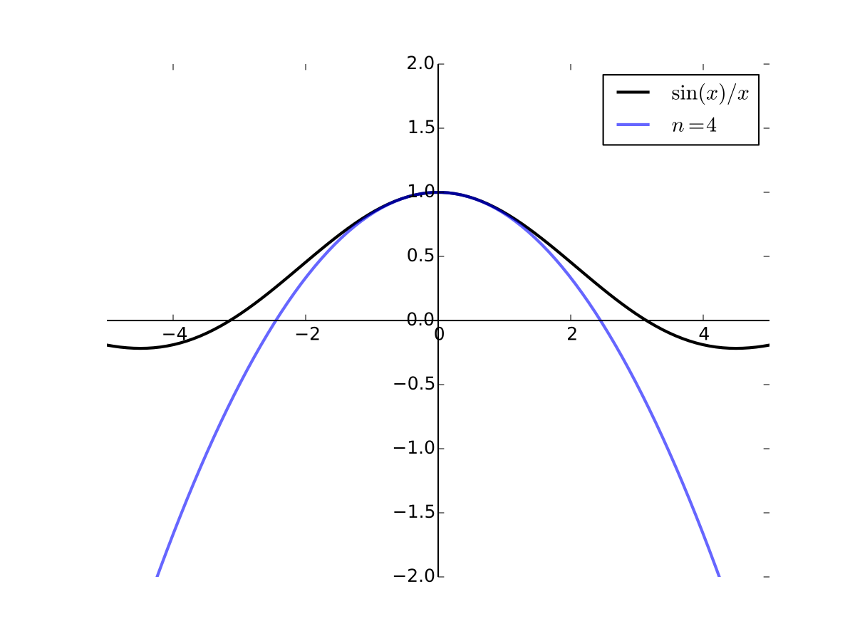
_images/taylor_4.png — Fig. 27 4th order Taylor series for $f(x) = \sin(x)/x$ at 0#

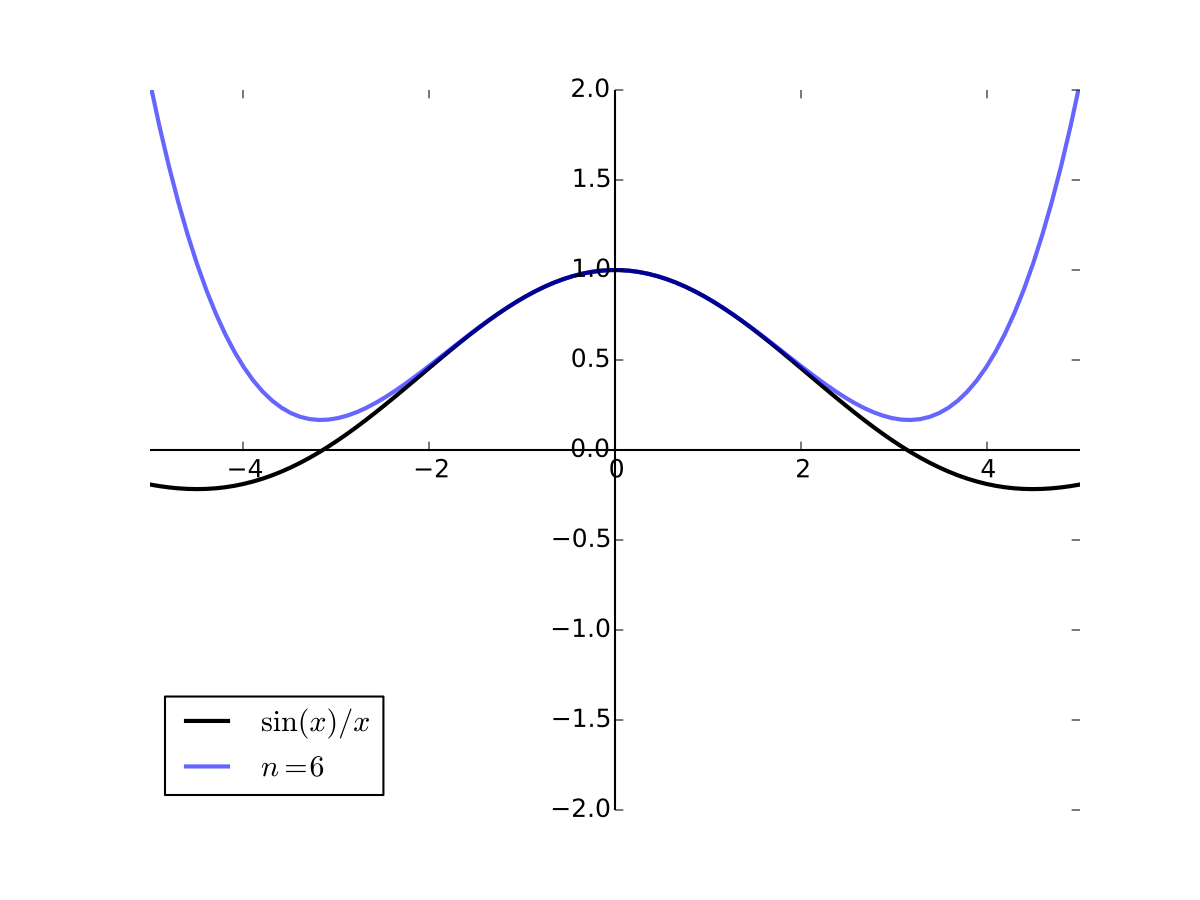
_images/taylor_6.png — Fig. 28 6th order Taylor series for $f(x) = \sin(x)/x$ at 0#

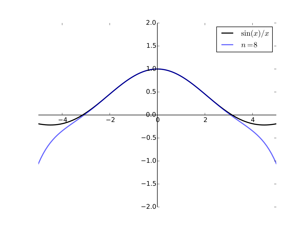
_images/taylor_8.png — Fig. 29 8th order Taylor series for $f(x) = \sin(x)/x$ at 0#

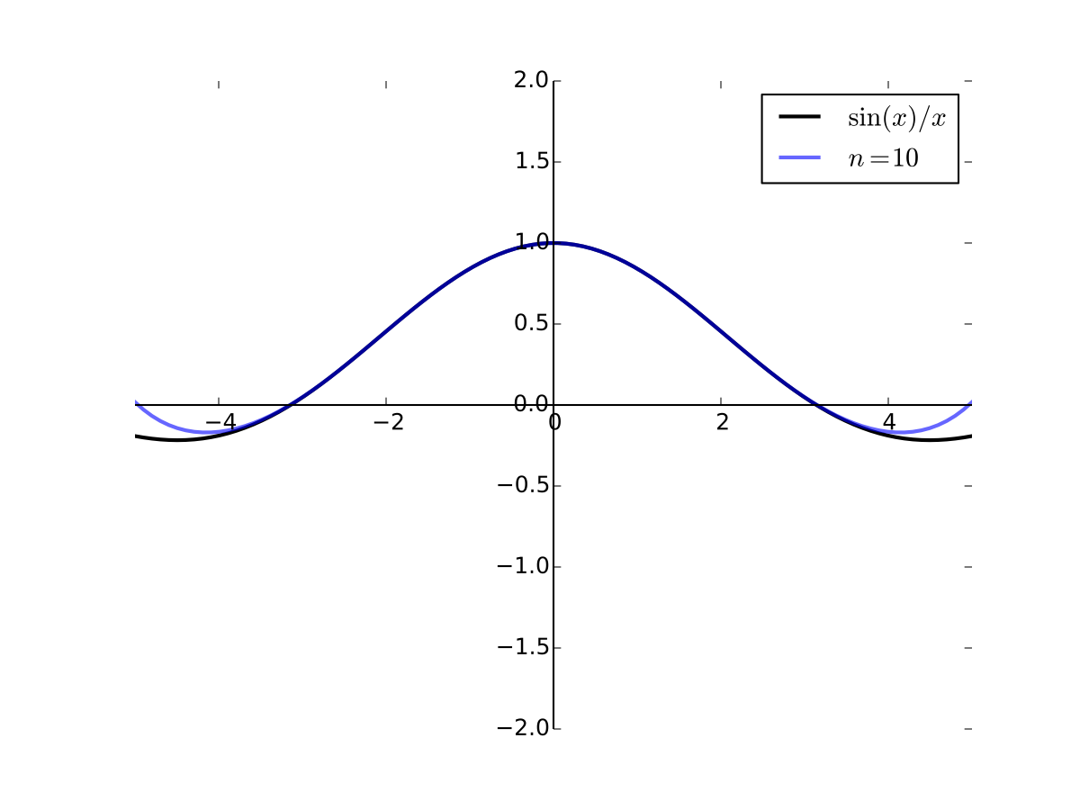
_images/taylor_10.png — Fig. 30 10th order Taylor series for $f(x) = \sin(x)/x$ at 0#

L’Hopital’s rule#

Consider the function $f(x)=\frac{g(x)}{h(x)}$.

Definition

If $\lim _{x \rightarrow x_{0}} g(x)=\lim _{x \rightarrow x_{0}} h(x)=0$, we call this situation an “$\frac{0}{0}$” indeterminate form

If $\lim _{x \rightarrow x_{0}} g(x)= \pm \infty$, $\lim _{x \rightarrow x_{0}} h(x)= \pm \infty$, we call this situation an “$\frac{ \pm \infty}{ \pm \infty}$” indeterminate form

Fact: L’Hopital’s rule for limits of indeterminate form

Suppose that $g(x)$ and $h(x)$ are both differentiable at all points on a non-empty interval $(a, b)$ that contains the point $x=x_{0}$, with the possible exception that they might not be differentiable at the point $x_{0}$.

Suppose also that $h^{\prime}(x) \neq 0$ for all $x \in(a, b)$.

Further, assume that for $f(x)=\frac{g(x)}{h(x)}$ we have either “$\frac{0}{0}$” or “$\frac{ \pm \infty}{ \pm \infty}$” indeterminate form.

Then if $\lim _{x \rightarrow x_{0}}\frac{g^{\prime}(x)}{h^{\prime}(x)}$ exists, then

\[ \lim _{x \rightarrow x_{0}} f(x) = \lim _{x \rightarrow x_{0}}\frac{g(x)}{h(x)} = \lim _{x \rightarrow x_{0}}\frac{g^{\prime}(x)}{h^{\prime}(x)} \]

all four conditions have to hold for the L’Hopital’s rule to hold!

Example

Note that in the examples below we have “$\frac{0}{0}$” indeterminacy, and both enumerator and denominator functions are differentiable around $x=0$

\[ \lim_{x \to 0} \frac{\ln(x+1)}{x} = \lim_{x \to 0} \frac{\frac{1}{x+1}}{1} = \lim_{x \to 0} \frac{1}{x+1} = 1 \]

\[ \lim_{x \to 0} \frac{e^x-1}{x} = \lim_{x \to 0} \frac{e^x}{1} = e^0 = 1 \]

Example

L’Hopital’s rule is not applicable for $\lim_{x \to 0} \frac{x}{\ln(x)}$ because neither “$\frac{0}{0}$” nor “$\frac{ \pm \infty}{ \pm \infty}$” indeterminacy form applies.

Some economic applications of derivatives#

Marginal revenue and marginal cost#

If a firm’s total revenue as a function of output is given by the function $R(Q)$, then its marginal revenue is given by the first derivative of that function:

\[ MR(Q)=\frac{d R(Q)}{d Q}=R^{\prime}(Q) \]

If a firm’s total cost as a function of output is given by the function $C(Q)$, then its marginal cost is given by the first derivative of that function:

\[ MC(Q)=\frac{d C(Q)}{d Q}=C^{\prime}(Q) \]

Interpretation of marginal values: change (in $R$ of $C$) caused by a small (infinitesimal) change in the variable $Q$.

Often interpreted as a changed caused by the unit change in the variable, using linear Taylor approximation.

Marginal revenue for a monopolist#

Consider a single-priced monopolist that faces an inverse demand curve that is given by the function $P(Q)$. Since demand curves usually slope down, we will assume that $P^{\prime}(Q)<0$. The total revenue for this monopolist is given by $R(Q)=P(Q) Q$. As such, the marginal revenue for this monopolist is

\[\begin{split} \begin{aligned} M R(Q) & =R^{\prime}(Q) \\ & =P^{\prime}(Q) Q+(1) P(Q) \\ & =P^{\prime}(Q) Q+P(Q) \\ & =P(Q)+P^{\prime}(Q) Q \\ & <P(Q) \end{aligned} \end{split}\]

Since $P(Q)$ will be the market price when the monopolist produces $Q>0$ units of output and $P^{\prime}(Q)<0$, we know that marginal revenue is less than the market price for a monopolist.

The two terms that make up marginal revenue for a monopolist can be given a very intuitive explanation. If the monopolist increases its output by a small amount, it receives the market price for the additional output (hence the $P(Q)$ term), but it loses some revenue due to the lower price that it will receive for all of the pre-existing output (the $P^{\prime}(Q) Q$ term).

Point elasticities#

Definition (in words)

Suppose that $y=f(x)$. The elasticity of $y$ with respect to $x$ is defined to be the percentage change in $y$ that is induced by a small (infinitesimal) percentage change in $x$.

So, what is a percentage change in $x$?

$x$ to $x+h$, making $h$ the absolute change in $x$
$x$ to $x + rx$, making $(x+rx)/x = 1+r$ the relative change in $x$, and $r$ is the relative change rate
percentage change in $x$ is the relative change rate expressed in percentage points

We are interested in infinitesimal percentage change, therefore in the limit as $r \to 0$ (irrespective of the units of $r$)

What is the percentage change in $y$?

Answer: rate of change of $f(x)$ that can be expressed as

\[ \frac{f(x+rx)}{f(x)} -1 = \frac{f\big(x(1+r)\big)-f(x)}{f(x)} \]

Let’s consider the limit

\[ \lim_{r \to 0} \frac{\frac{f\big(x(1+r)\big)-f(x)}{f(x)}}{r} = \frac{1}{f(x)} \lim_{r \to 0} \frac{f\big(x(1+r)\big)-f(x)}{r} = \]

Define a new function $g$ such that $f(x) = g\big(\ln(x)\big)$ and $f\big(x(1+r)\big) = g\big(\ln(x) + \ln(1+r)\big)$

Continuing the above, and noting that $\ln(1+r) \to 0$ as $r \to 0$ we have

\[\begin{split} \begin{array}{l} = \frac{1}{f(x)} \lim_{r \to 0} \frac{g\big(\ln(x) + \ln(1+r)\big)-g\big(\ln(x)\big)}{r} = \\ = \frac{1}{f(x)} \lim_{r \to 0} \frac{g\big(\ln(x) + \ln(1+r)\big)-g\big(\ln(x)\big)}{\ln(1+r)} \frac{\ln(1+r)}{r} = \\ = \frac{1}{f(x)} \left[ \lim_{r \to 0} \frac{g\big(\ln(x) + \ln(1+r)\big)-g\big(\ln(x)\big)}{\ln(1+r)} \lim_{r \to 0} \frac{\ln(1+r)}{r} \right] =\\= \frac{1}{f(x)} \frac{d g(\ln(x))}{d \ln(x)} = \frac{1}{f(x)} \frac{d f(x)}{d \ln(x)} = \frac{x}{f(x)} \frac{d f(x)}{d x} \end{array} \end{split}\]

See the example above showing that $\lim_{r \to 0} \frac{\ln(1+r)}{r} = 1$.

In the last step, to make sense of the expression $\frac{d f(x)}{d \ln(x)}$, imagine that $x$ is a function of some other variable we call $\ln(x)$. Then we can use the chain rule and the inverse function rule to show that

\[ \frac{d f(x)}{d \ln(x)} = \frac{d f(x)}{d x} \frac{dx}{d \ln(x)} = \frac{d f(x)}{d x} \frac{1}{\frac{1}{x}} = x \frac{d f(x)}{d x} \]

Note, in addition, that by the chain rule the following also holds

\[ \frac{d \ln f(x)}{d \ln(x)} = \frac{1}{f(x)} \frac{d f(x)}{d \ln(x)} \]

Putting everything together, we arrive at the following equivalent expressions for elasticity.

Definition (exact)

The (point) elasticity of $f(x)$ with respect to $x$ is defined to be the percentage change in $y$ that is induced by a small (infinitesimal) percentage change in $x$, and is given by

\[ \epsilon^{f}_{x}(x)= \lim_{r \to 0} \frac{\frac{f\big(x(1+r)\big)}{f(x)}-1}{r} = \frac{\frac{d f(x)}{d x}}{\frac{f(x)}{x}} = \frac{x}{f(x)} \frac{d f(x)}{d x} = \frac{d \ln f(x)}{d \ln x} \]

Example

Suppose that we have a linear demand curve of the form

\[ Q = a − bP \]

where $a > 0$ and $b > 0$ The slope of this demand curve is equal to $(−b)$ As such, the point own-price elasticity of demand in this case is given by

\[\begin{split} \begin{align*} \epsilon^D_P (P) &= \left( \frac{P}{a - bP} \right) (-b) \\ &= \left( \frac{-bP}{a - bP} \right) \end{align*} \end{split}\]

Note that

\[\begin{split} \begin{align*} | \epsilon^D_P (P) | &= 1 \\ \iff | \frac{-bP}{a - bP} | &= 1 \\ \iff \frac{bP}{a - bP} &= 1 \\ \iff bP &= a - bP \\ \iff 2bP &= a \\ \iff P &= \frac{a}{2b} \\ \end{align*} \end{split}\]

More generally, we can show that, for the linear demand curve above, we have

\[\begin{split} | \epsilon^D_P (P) | = \begin{cases} \in (0, 1) \;\; \text{ if } P < \frac{a}{2b} \\ = 1 \;\; \text{ if } P = \frac{a}{2b} \\ \in (1, \infty) \;\; \text{ if } P > \frac{a}{2b} \\ \end{cases} \end{split}\]

Since the demand curve above is downward sloping, this means that

\[\begin{split} \epsilon^D_P (P) = \begin{cases} \in (-1, 0) \;\; \text{ if } P < \frac{a}{2b} \\ = -1 \;\; \text{ if } P = \frac{a}{2b} \\ \in (-\infty, -1) \;\; \text{ if } P > \frac{a}{2b} \\ \end{cases} \end{split}\]

Example

Suppose that we have a demand curve of the form

\[ Q = a/P \]

where $a > 0$. Computing the point elasticity of demand at price $P$ we have

\[\begin{split} \begin{align*} \epsilon^D_P (P) &= \left( \frac{P}{a/P} \right) \left( \frac{-a}{P^2} \right) \\ &= \frac{P^2}{a}\frac{-a}{P^2} = -1 \end{align*} \end{split}\]

Constant own-price elasticity!

Alternatively we could compute this elasticity as

\[\begin{split} Q &= a/P = a P^{-1} \quad \Leftrightarrow \quad \ln Q = \ln a - \ln P \\ \epsilon^D_P (P) &= \frac{d \ln Q}{d \ln P} = -1 \end{split}\]

Notes from the lecture#

Hand written notes from the lecture

📖 Univariate differentiation

Contents

📖 Univariate differentiation#

Sources and reading guide#

Limit for functions#

The structure of \(\epsilon–\delta\) arguments#

Heine and Cauchy definitions of the limit for functions#

Some useful rules about limits#

Continuity#

Types of discontinuities#

Derivatives#

Definition#

The binomial theorem

Some useful differentiation rules#

The quotient rule is redundant#

Differentiability and continuity#

Continuity does NOT imply differentiability#

Differentiability implies continuity#

Higher-order derivatives#

Taylor series#

L’Hopital’s rule#

Some economic applications of derivatives#

Marginal revenue and marginal cost#

Marginal revenue for a monopolist#

Point elasticities#

Notes from the lecture#