📖 Univariate integration

Announcements & Reminders

Online Test 5 on Monday May 20
- 30 minutes, open book
- 10% of the final grade
The final exam
- Friday May 31, 2pm
- 3 hours exam + 15 minutes reading time
- closed book, no materials allowed
- Manning Clark Hall, room 1.04, Cultural Centre Kambri
Tutorials replaced by consultations in week 12
- Same schedule and locations
- Questions and answers
- You can come to multiple sessions through the week
My consultation hours
- Wednesday May 22, 9:30-11:00
- Office 1021, HW Arndt Building
- Come with specific questions
Next lecture: revision and consultation
- 1/2 revision and exemplar exam problem
- 1/2 questions and answers
- Free participation
Feedback
- Very important
- Don’t miss SELT feedback forms
- Evaluate your convener, all lecturers and your tutor

📖 Univariate integration#

⏱ | words

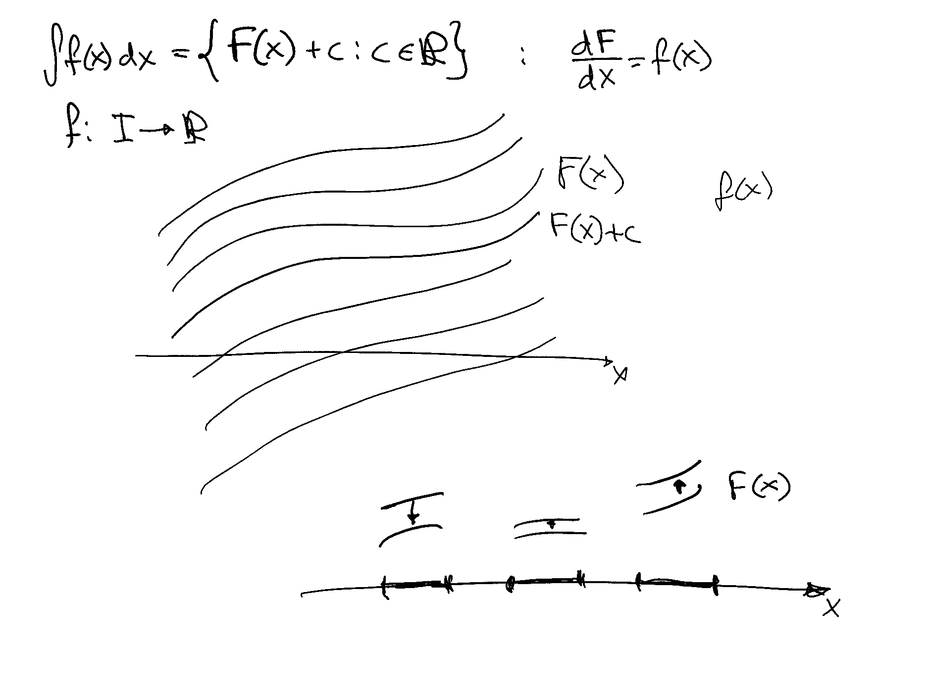
Anti-derivative#

Definition

Let \(I=(a, b)=\{x \in \mathbb{R}: a<x<b\}\) wherea \(\in \mathbb{R}, b \in \mathbb{R}\), and \(a<b\)

Let \(f: I \to \mathbb{R}\) be some univariate real-valued function. Suppose that there exists some function \(F: I \to \mathbb{R}\) such that

\[ F^{\prime}(x)=\frac{d F(x)}{dx}=f(x) \text { for all } x \in I \]

In this case, the function \(F(x)\) is called an anti-derivative of the function \(f(x)\) on the interval \(I\)

Note that \(I \in \mathbb{R}\) is a non-empty open interval of real numbers that contains more than a single point

Example

\[ f(x) = 3x^2 + 4x + 1 \quad \implies \quad F(x) = x^3 + 2x^2 + x + 5 \; \text{ is anti-derivative} \]

\[ f(x) = \exp(x) \quad \to \quad F(x) = exp(x)-1 \; \text{ is anti-derivative} \]

Anti-derivatives are NOT unique#

If the function \(F(x)\) is an anti-derivative of the function \(f(x)\) on the interval \(I\), then so is the function \(G(x)=F(x)+C\), where \(C \in \mathbb{R}\) is some fixed real number.

This can be seen by differentiating \(G(x)\) with respect to \(x\). Upon doing this, we obtain

\[ \frac{d}{dx}(F(x)+C)=\frac{d F(x)}{dx}+\frac{d C}{dx}=f(x)+0=f(x) \]

The constant \(C \in \mathbb{R}\) is known as an arbitrary constant because it can take the form of any given real number. In effect, if the function \(F(x)\) is an anti-derivative of the function \(f(x)\) on the interval \(I\), then there is an entire family of such anti-derivatives of \(f(x)\) on the interval \(I\). This family is given by the set

\[ \{F(x)+C: C \in \mathbb{R}\} \]

Indefinite integral#

Definition

Suppose that the function \(F(x)\) is an anti-derivative of the function \(f(x)\) on the connected open interval \(I\).

The indefinite integral of \(f(x)\), denoted by \(\int f(x) dx\), is the set of all anti-derivatives of fucntion \(f(x)\)

\[ \int f(x) dx = \{ F(x)+C: C \in \mathbb{R} \} \]

Note, however, that it is common to drop the set notation and simply use the integral sign to denote a generic member of the set of all anti-derivatives of \(f(x)\) on the interval \(I\).

In other words, the indefinite integral of \(f(x)\) on the interval \(I\) is

\[ \int f(x) dx = F(x)+C \]

where \(C \in \mathbb{R}\) is an arbitrary constant. Note that here, the arbitrary constant \(C\) is interpreted as being truly arbitrary, rather than taking on a particular value

Note that we mention that interval \(I\) is connected. If it was not we could have different arbitrary constants for different parts of the domain, and thus the above expression with a single constant \(C\) would not be valid

Example(quick exercise)

\[ f(x)=0 \quad \int f(x) dx = \int 0 dx = \text{?} \]

\[ f(x)=5 \quad \int f(x) dx = \int 5 dx = \text{?} \]

\[ f(x)=x \quad \int f(x) dx = \int x dx = \text{?} \]

\[ f(x)=6 x^2 \quad \int f(x) dx = \int 6 x^2 dx = \text{?} \]

\[ f(x)=\frac{1}{x} \quad \int f(x) dx = \int \frac{1}{x} dx = \text{?} \]

Some terminology

Suppose that \(f: I \to \mathbb{R}\), where \(I \subseteq \mathbb{R}\) is a connected open interval, and \(F^{\prime}(x)=f(x)\) for all \(x \in I\)

\(\int f(x) dx=F(x)+C\) is the indefinite integral of \(f(x)\)
\(f(x)\) is the integrand
\(dx\) means “with respect to \(x\) “, \(x\) is the variable of integration
\(F(x)\) is an anti-derivative of \(f(x)\)
\(C\) is an arbitrary constant

Properties of indefinite integral#

Fact

Suppose that \(f: I \to \mathbb{R}\) is at least once continuously differentiable on \(I\), where \(I \subseteq \mathbb{R}\) is a connected open interval, and \(F^{\prime}(x)=f(x)\) for all \(x \in I\). Then for any constant \(k \ne 0\)

\[ \int k f(x) dx = k \int f(x) dx = k F(x)+C \]

A constant can be taken outside of the integral

Proof

Informal proof
Note that

\[\begin{split} \begin{aligned} \frac{d}{dx}(k F(x)+C)&=\frac{d}{dx} k F(x)+\frac{d}{dx} C \\ & =k \frac{d}{dx} F(x)+0 \\ & =\quad k F^{\prime}(x) \\ & =\quad k f(x) \end{aligned} \end{split}\]

Note also that

\[ k \int f(x) dx=k\left(F(x)+C_{f}\right)=k F(x)+k C_{f}=k F(x)+C \]

where \(C_{f}\) and \(C=k C_{f}\) are arbitrary constants. \(\blacksquare\)

Fact

Suppose that \(f: I \to \mathbb{R}\) and \(g: I \to \mathbb{R}\) are both at least once continuously differentiable on \(I\), where \(I \subseteq \mathbb{R}\) is a connected open interval

\[ \int[f(x)+g(x)] dx=\int f(x) dx+\int g(x) dx=F(x)+G(X)+C \]

together with the previous fact, we establish linearity of indefinite integrals in the space in a certain vector space of functions

Proof

Informal proof
Note that

\[\begin{split} \begin{aligned} \frac{d}{dx}(F(x)+G(x)+C) & =\frac{d}{dx} F(x)+\frac{d}{dx} G(x)+\frac{d}{dx} C \\ & =F^{\prime}(x)+G^{\prime}(x)+0 \\ & =f(x)+g(x) \end{aligned} \end{split}\]

Note also that \(\int f(x) dx=F(x)+C_{f}\) and \(\int g(x) dx=G(x)+C_{g}\), so that

\[ \int f(x) dx+\int g(x) dx=F(x)+C_{f}+G(x)+C_{g}=F(x)+G(x)+C \]

where \(C_{f}, C_{g}\), and \(C=C_{f}+C_{g}\) are arbitrary constants. \(\blacksquare\)

Together the previous two facts establish the following result

Fact

Suppose that the functions \(f_{i}: I \to \mathbb{R}, i \in\{1,2, \cdots, n\}\), are all at least once continuously differentiable on \(I\), where \(I \subseteq \mathbb{R}\) is a connected open interval. Suppose also that \(k_{i} \in \mathbb{R}, i \in\{1,2, \cdots, n\}\), are some given constants, and \(C \in \mathbb{R}\) is an arbitrary constant Suppose as well that \(F_{i}^{\prime}(x)=f_{i}(x)\) for all \(x \in I\) and for each \(i \in\{1,2, \cdots, n\}\) The following formula applies to \(\left\{f_{i}(x)\right\}_{i=1}^{n}\)

\[\begin{split} \begin{aligned} & \int\left[\sum_{i=1}^{n} k_{i} f_{i}(x)\right] dx=\sum_{i=1}^{n}\left[\int k_{i} f_{i}(x) dx\right] \\ & =\sum_{i=1}^{n}\left[k_{i} \int f_{i}(x) dx\right]=\sum_{i=1}^{n} k_{i} F_{i}(x)+C \end{aligned} \end{split}\]

Proof

Proof by a repeated application of the previous two facts

Fact

Suppose that \(f: I \to \mathbb{R}\) is at least once continuously differentiable on \(I\), where \(I \subseteq \mathbb{R}\) is a connected open interval

\[ \frac{d}{dx} \int f(x) dx=f(x) \]

and

\[ \int f^{\prime}(x) dx=f(x)+C \]

Proof

The fact follows from the definition of the indefinite integral and the anti-derivative.

First formula:

Suppose that \(F(x)\) is an anti-derivative of \(f(x)\)
This means that \(\int f(x)=F(x)+C\)
Clearly, we must have \(\frac{d}{dx} \int f(x)=\frac{d}{dx}(F(x)+C)\)
But \(\frac{d}{dx}(F(x)+C)=\frac{d}{dx} F(x)+0=\frac{d}{dx} F(x)=f(x)\), because \(F(x)\) is an anti-derivative of \(f(x)\) and \(C\) is an (albeit arbitrary) constant
Thus we have \(\frac{d}{dx} \int f(x) dx=f(x)\)

Second formula:

Suppose that \(f(x)\) is at least once continuously differentiable, and denote its derivative by \(f^{\prime}(x)\)
Let \(F(x)=f(x)+C\), where \(C\) is an arbitrary constant
Clearly we must have \(\frac{d}{dx} F(x)=\frac{d}{dx} f(x)+0=\frac{d}{dx} f(x)=f^{\prime}(x)\)
Furthermore, we have already shown that \(\frac{d}{dx} \int g(x) dx=g(x)\). This means that we must have \(\frac{d}{dx} \int f^{\prime}(x) dx=f^{\prime}(x)\)
Thus we have \(\frac{d}{dx} \int f^{\prime}(x) dx=\frac{d}{dx} F(x)\),
Upon integrating both sides of this equation, we obtain \(\int f^{\prime}(x) dx=F(x)\), so that we have \(\int f^{\prime}(x) dx=f(x)+C\)

\(\blacksquare\)

Examples

\[ \int \big[6x^2 + \exp(x) \big] dx = 6 \int x^2 dx + \int \exp(x) dx = 2 x^3 + \exp(x) + C \]

\[\begin{split} \frac{d}{dx} \int \frac{1}{x} dx = \frac{d}{dx} \big[ \ln(|x|) + C\big] = \frac{1}{x} = \begin{cases} \frac{1}{x}, & x > 0 \\ - \frac{1}{-x}, & x < 0 \end{cases} \end{split}\]

Integration zoo#

The list of most common integrals

Fact

\[ \int k dx=k x+C \]

\[ \int x^{n} dx=\frac{x^{n+1}}{n+1}+C \]

\[ \int x^{-1} dx=\ln|x|+C \]

\[ \int \exp^x dx=\exp^x+C \]

\[ \int a^x dx=\frac{a^x}{\ln a}+C \]

\[ \int \ln x dx=x \ln x -x +C \]

Integration techniques#

There are a number of techniques that can be used to find the indefinite integral of a function

Direct integration#

This technique involves recognising that the integrand is the derivative of a particular function, or, rather, class of functions. It is most useful when the integrand is an elementary function.

Direct integration makes use of the fact that if \(F^{\prime}(x)=f(x)\), then the indefinite integral of \(f(x)\) is given by \(\int f(x) dx=F(x)+C\)

Example

Since \(\frac{d}{dx} x^{\alpha}=\alpha x^{\alpha-1}\), we have \(\int \alpha x^{\alpha-1} dx=x^{\alpha}+C\)

Since \(\frac{d}{dx} e^{a x}=a e^{a x}\), we have \(\int a e^{a x} dx=e^{a x}+C\)

Let \(x \in(0, \infty)\). Since \(\frac{d}{dx} \ln (x)=\frac{1}{x}\), we have \(\int \frac{1}{x} dx=\ln (x)+C\)

Integration by substitution#

This is the integration counterpart to the chain rule of differentiation.

Suppose that \(F:(a, b) \to \mathbb{R}\) be a function that is differentiable on the interval \((a, b) \subseteq \mathbb{R}\) and let \(f(x)=F^{\prime}(x)\). So, \(\int f(x) dx = F(x) + C\).

Suppose that \(\omega:(c, d) \to(a, b)\) be a function that is differentiable on the interval \((c, d) \subseteq \mathbb{R}\)

Consider the composite function \(G=F \circ \omega: (c, d) \to \mathbb{R}\) defined by \(G(t)=F(\omega(t))\)

Differentiating both function, and using the chain rule of differentiation we have

\[ G'(t) = \frac{d}{dt} F(\omega(t)) = F'(\omega(t)) \omega'(t) = f(\omega(t))\omega'(t) \]

By definition of anti-derivative it follows that

\[ G(t)+ C = \int G'(t) dt = \int f(\omega(t))\omega'(t) dt \]

On the other hand, when \(x=\omega(t)\), \(G(t)=F(x)\), and thus

\[ \int f(x) dx = F(x)+C = G(t)+C = \int f(\omega(t))\omega'(t) dt \]

We now have a framework for discussing the technique of integration by substitution. This techniques is useful in circumstances where each of the following properties is true:

You do not know how to calculate the indefinite integral of \(f(x)\) with respect to \(x\)
You can see a way to express \(f(x)\) as \(f(x)=g(\omega(t)) \omega^{\prime}(t)\) for which you know the functions \(g(x)\) and \(\omega(t)\)
You do know how to calculate the indefinite integral of \(g(x)\) with respect to \(x\)

Fact

Suppose that \(f: I \to \mathbb{R}\) is at least once continuously differentiable on \(I\), where \(I \subseteq \mathbb{R}\) is a connected open interval, and let \(\omega : \Omega \to I\), where \(\Omega \subseteq \mathbb{R}\), be a differentiable function, then:

\[ \int f(x) dx = \int f(\omega(t)) \omega^{\prime}(t) dt \]

Example

\[ \int f(x) dx = \int \frac{\ln (x)}{x} dx = \]

Let’s make a substitution \(t = \ln(x)\), in which case \(x=\exp(t)=\omega(t)\) and \(\omega'(t)=\exp(t)\). We continue

\[\begin{split} = \int \frac{\ln (\omega(t))}{\omega(t)}\omega'(t) dt = \int \frac{\ln (\exp(t))}{\exp(t)}\exp(t) dt = \\ \int t dt = t^2/2 + C = (\ln(x))^2/2 + C \end{split}\]

As a check of our solution, note that

\[\begin{split} \begin{gathered} \frac{d}{dx}\left(\frac{\ln ^{2}(x)}{2}\right)=\left(\frac{1}{2}\right)(2) \ln (x)\left(\frac{d \ln (x)}{dx}\right) \\ \quad=(1) \ln (x)\left(\frac{1}{x}\right)=\frac{\ln (x)}{x}=f(x) \end{gathered} \end{split}\]

Example

\[ \int f(x) dx=\int e^{x^{2}} x dx = \]

Let use a new variable \(t=x^2\), in other words \(x=\sqrt{t}=\omega(t)\), \(\omega'(t) = \frac{1}{2\sqrt{t}}\). Continuing

\[ = \int e^{t} \sqrt{t} \frac{1}{2\sqrt{t}} dt = \frac{1}{2} \int e^{t} dt = \frac{1}{2} e^{t} +C = \frac{1}{2} e^{x^2} +C \]

As a check we have

\[ \frac{d}{dx}\left(\frac{1}{2} e^{x^{2}}\right)=\frac{1}{2}(2 x) e^{x^{2}}=x e^{x^{2}}=e^{x^{2}} x \]

Integration by parts#

This is the integration counterpart to the product rule of differentiation.

Suppose that \(u:(a, b) \to \mathbb{R}\) and \(v:(a, b) \to \mathbb{R}\) are both functions that are differentiable on the interval \((a, b) \subseteq \mathbb{R}\)

Consider the function \(J:(a, b) \to \mathbb{R}\) defined by \(J(x)=u(x) v(x)\) We know from the product rule of differentiation that

\[ \frac{d}{dx}(u(x) v(x))=u^{\prime}(x) v(x)+v^{\prime}(x) u(x) \]

This expression can be rearranged to obtain

\[ u^{\prime}(x) v(x)=\frac{d}{dx}(u(x) v(x))-v^{\prime}(x) u(x) \]

And since the two functions in the RHS and the LHS are equal, so are their anti-derivatives

\[\begin{split} \begin{gathered} \int u^{\prime}(x) v(x) dx=\int\left(\frac{d}{dx}(u(x) v(x))-v^{\prime}(x) u(x)\right) dx \\ =\int \frac{d}{dx}(u(x) v(x)) dx-\int v^{\prime}(x) u(x) dx \end{gathered} \end{split}\]

We already know that

\[ \int \frac{d}{dx}(u(x) v(x)) dx=u(x) v(x)+C \]

where \(C \in \mathbb{R}\) is an arbitrary constant, and therefore we have

\[ \int u^{\prime}(x) v(x) dx=u(x) v(x)-\int v^{\prime}(x) u(x) dx+C \]

Note that \(\int u^{\prime} v dx\) and \(\int v^{\prime} u dx\) both implicitly incorporate arbitrary constants If we absorb the explicit arbitrary constant \((C)\) in the above expression into the implicity arbitrary constants in the \(\int u^{\prime} v dx\) and \(\int v^{\prime} u dx\) terms in some appropriate fashion, then we can rewrite that expression as

\[ \int u^{\prime}(x) v(x) dx=u(x) v(x)-\int v^{\prime}(x) u(x) dx \]

This expression forms the foundation for the integration technique known as integration by parts. Clearly, integration by parts is the integral counterpart to the product rule of differentiation

Integration by parts is particularly useful when you want to find \(\int f(x) dx=\int u^{\prime} v dx\) and either of the following two situations occur

The indefinite integral \(\int v^{\prime} u dx\) is easier to obtain than the indefinite integral \(\int u^{\prime} v dx\)
It turns out that \(\int v^{\prime} u dx=\mathrm{k} \int u^{\prime} v dx\) for some constant \(k \in \mathbb{R}\). (In this case, you get a functional equation in which the “variable” is the integrand \(\int u^{\prime} v dx\). This equation can then be solved to obtain integrand \(\int u^{\prime} v dx\)

Sometimes, you might need to undertake multiple iterations of the technique of integration by parts

Fact

Suppose that \(u,v: I \to \mathbb{R}\) is at least once continuously differentiable on \(I\), where \(I \subseteq \mathbb{R}\) is a connected open interval. Then

\[ \int u'(x) v(x) dx = u(x) v(x) - \int v'(x) u(x) dx \]

Example

We want to find \(\int \ln (x) dx\) Let \(u(x)=x\) and \(v(x)=\ln (x)\). This means that \(u^{\prime}(x)=1\) and \(v^{\prime}(x)=\frac{1}{x}\) This allows us to express the required integral as

\(\int \ln (x) dx=\int(1) \ln (x) dx=\int u^{\prime}(x) v(x) dx\)

Integrating by parts, and ignoring any arbitrary constants, we obtain

\[ \int \ln (x) dx=x \ln (x)-\int\left(\frac{1}{x}\right) x dx=x \ln (x)-\int dx=x \ln (x)-x \]

Thus we can conclude that

\[ \int \ln (x) dx=x \ln (x)-x+C \]

where \(C \in \mathbb{R}\) is an arbitrary constant

Example

We want to find \(\int \frac{\ln (x)}{x} dx\) Let \(u(x)=\ln (x)\) and \(v(x)=\ln (x)\). This means that \(u^{\prime}(x)=\frac{1}{x}\) and \(v^{\prime}(x)=\frac{1}{x}\) This allows us to express the required integral as \(\int \frac{\ln (x)}{x} dx=\int u^{\prime}(x) v(x) dx\)

Integrating by parts, and ignoring any arbitrary constants, we obtain

\[\begin{split} \begin{gathered} \int \frac{\ln (x)}{x} dx=\int u^{\prime}(x) v(x) dx=u(x) v(x)-\int v^{\prime}(x) u(x) dx \\ =(\ln (x))(\ln (x))-\int \frac{\ln (x)}{x} dx=(\ln (x))^{2}-\int \frac{\ln (x)}{x} dx \\ =\ln ^{2}(x)-\int \frac{\ln (x)}{x} dx \end{gathered} \end{split}\]

Ignoring any arbitrary constants, we have shown that

\[ \int \frac{\ln (x)}{x} dx=\ln ^{2}(x)-\int \frac{\ln (x)}{x} dx \]

This equation can be rearranged to obtain

\[ 2 \int \frac{\ln (x)}{x} dx=\ln ^{2}(x) \]

so that, ignoring any arbitrary constants, we have

\[ \int \frac{\ln (x)}{x} dx=\left(\frac{1}{2}\right) \ln ^{2}(x) \]

Thus we know that

\[ \int \frac{\ln (x)}{x} dx=\left(\frac{1}{2}\right) \ln ^{2}(x)+C \]

where \(C \in \mathbb{R}\) is an arbitrary constant

Definite integral#

It’s all about the area under the curve!

How might we try and measure the area under a curve? One way might be to try and approximate it by adding up the area of boxes whose sum seems like it should be close to the area under the curve The advantage of this approach is that calculating the area of boxes (or, rather rectangles) is easy. We know from high school (and perhaps even primary school) that it is just length times breadth (or height times width)

Definition

A finite partition of an interval \([a,b] \subset \mathbb{R}\) is a finite set of points \(T_n = \left\{t_{0}, t_{1}, t_{2}, \cdots, t_{n-1}, t_{n} \right\}\) such that \(a=t_{0}<t_{1}<t_{2}<\cdots<t_{n-1}<t_{n}=b\)

Let \(r(T_n)=r(t_{0},t_{1},\cdots,t_{n-1},t_{n}) = \max_{0\leq i \leq n-1}(t_{i+1}-t_{i})\) denote the norm of the partition

note that the partition covers the whole interval: \(\left[a, t_{1}\right] \cup\left(t_{1}, t_{2}\right] \cup\left(t_{2}, t_{3}\right] \cup \cdots \cup\left(t_{n-1}, t_{n}\right] \cup\left(t_{n}, b\right]=[a, b]\)
and the sub-intervals are disjoint \(\left[a, t_{1}\right] \cap\left(t_{1}, t_{2}\right] \cap\left(t_{2}, t_{3}\right] \cap \cdots \cap\left(t_{n-1}, t_{n}\right] \cap\left(t_{n}, b\right]=\varnothing\)

We can use this partition to form the bases of \(n\) rectangles. The bases are given by the sub-intervals, and the heights are given by the function values at the interval.

Which function values should we use? The left end-point, the right end-point, or the mid-point?

Definition (Riemann sum)

Let \(f: [a,b] \to \mathbb{R}\) be a function defined on a connected interval \([a,b] \subset \mathbb{R}\), and let \(T = \left\{t_{0}, t_{1}, t_{2}, \cdots, t_{n-1}, t_{n} \right\}\) be a partition of the interval \([a,b]\) with norm \(r(T)\).

The Riemann sum is the sum of the form

\[ S(T_n) = \sum_{i=1}^{n-1} f(x_i^{\star})(x_{i+1} - x_i), \quad x_i^{\star} \in [x_i, x_{i+1}] \text{ for all } i=1,\dots,n-1 \]

In Riemann sums the choice of \(x_i^{\star}\) within each subinterval \([x_i, x_{i+1}]\) is free!

Definition (Darboux sums)

In the same settings, the upper and lower Darboux sums are giveb by

\[ U(T_n) = \sum_{i=1}^{n-1} \max_{x \in [x_i, x_{i+1}]}f(x)(x_{i+1} - x_i) \]

\[ L(T_n) = \sum_{i=1}^{n-1} \min_{x \in [x_i, x_{i+1}]}f(x)(x_{i+1} - x_i) \]

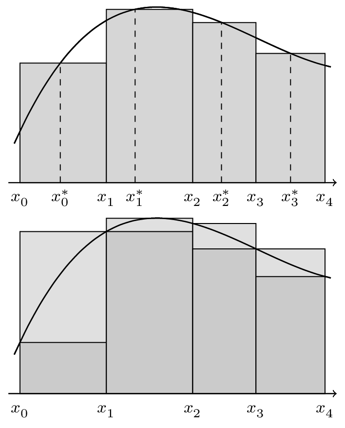
_images/lower_upper.png — Fig. 35 Riemann and Darboux lower and upper sums#

Definition

A function \(f: [a,b] \to \mathbb{R}\) is said to be Riemann integrable on \([a,b]\) if for any finite partition of \([a,b]\) which norm converges to zero, the limit of the difference of the Darboux upper and lower sums exists and is also equal to zero

\[ \lim_{n \to \infty} U(T_n)-L(T_n) = 0 \quad \text{for all} \quad T_n: \lim_{n \to \infty} r(T_n) = 0 \]

That is for any \(\epsilon > 0\) there exists a \(\delta > 0\) such that for any partition \(T_n\) with \(r(T_n) < \delta\) we have \(|U(T_n)-L(T_n)| < \epsilon\).

most of the functions we encounter in practice are Riemann integrable
in fact all functions which are continuous on \([a,b]\) at almost all points (except for a set of measure zero) are Riemann integrable

Example

An example of a function which is not Riemann integrable is \(f: \mathbb{R} \to \mathbb{R}\) defined as

\[\begin{split} f(x)= \begin{cases} 0, & x \in \mathbb{Q} \\ 1, & x \in \mathbb{R} \setminus \mathbb{Q} \end{cases} \end{split}\]

To see this, note that for any partition \(T_n\) we have \(U(T_n)-L(T_n) = 1\) because within any (open) interval on real line there are both rational and irrational numbers (where irrational are real which are not rational). Therefore the requisite limit does not exist and the function is not Riemann integrable.

Fact

If function \(f: [a,b] \to \mathbb{R}\) is Riemann integrable on \([a,b]\), there exists a unique number \(I_f(a,b) \in \mathbb{R}\) such that

\[ \lim_{n \to \infty} U(T_n) = \lim_{n \to \infty} L(T_n) = \lim_{n \to \infty} S(T_n) = I_f(a,b) \quad \text{for all} \quad T_n: \lim_{n \to \infty} r(T_n) = 0 \]

both Riemann and the two Darboux sums converge to the same value

Definition

Number \(I_f(a,b)\) from the previous fact is called the definite integral of \(f\) over \([a,b]\) and is denoted by

\[ \lim_{n \to \infty} S(T_n) = \int_{a}^{b} f(x) dx \quad \text{for all} \quad T_n: \lim_{n \to \infty} r(T_n) = 0 \]

This type of definite integral is known as a Riemann definite integral

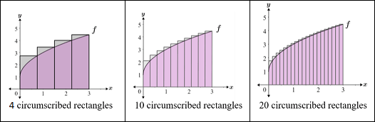
_images/riemann.png — Fig. 36 Limit of Riemann sums#

Example

Consider \(f(x) = \exp(x)\) on \([0,1]\). Let’s compute \(U(T_n)\), \(L(T_n)\) and \(S(T_n)\) for finite partitions of the interval with uniformly spaced \(n-1\) points. Because the function is increasing, the upper sum will be the sum of the function values at the right end-points of the subintervals, and the lower sum will be the sum of the function values at the left end-points of the subintervals, and we take midpoint for the Riemann sums.

import numpy as np
fun = lambda x: np.exp(x)
a,b = 0,1
print(f"{'n':<7} {'L(T_n)':>12} {'S(T_n)':>12} {'U(T_n)':>12}")
# for n in range(2, 1000, 10):
L,U,n=0,1,2
while np.abs(U - L) > 1e-5:
  x = np.linspace(a, b, n)     # partition (uniform)
  dx = x[1] - x[0]             # norm of the partition
  U = np.sum(fun(x[1:]) * dx)  # fun at right side
  L = np.sum(fun(x[:-1]) * dx) # fun at left side
  S = np.sum(fun((x[1:] + x[:-1]) / 2) * dx) # fun at midpoint
  print(f"{n:<7.0f} {L:>12.8f} {S:>12.8f} {U:>12.8f}")
  n *= 2

n             L(T_n)       S(T_n)       U(T_n)
       1.00000000   1.64872127   2.71828183
       1.44778216   1.71035252   2.02054276
       1.59846867   1.71682157   1.84393750
      1.66164212   1.71796367   1.77619424
      1.69071660   1.71820733   1.74614505
      1.70468075   1.71826379   1.73195506
     1.71152582   1.71827739   1.72505560
     1.71491485   1.71828073   1.72165321
     1.71660108   1.71828155   1.71996367
    1.71744214   1.71828176   1.71912179
    1.71786216   1.71828181   1.71870157
    1.71807203   1.71828182   1.71849164
    1.71817694   1.71828183   1.71838672
   1.71822939   1.71828183   1.71833427
   1.71825561   1.71828183   1.71830805
   1.71826872   1.71828183   1.71829494
131072    1.71827527   1.71828183   1.71828838
262144    1.71827855   1.71828183   1.71828511

Negative values of integrals#

What happens if \(f(x)<0\) for some \(x\)?

Definite integral is the aggregate signed area between the curve that represents the graph of that function and the axis for the independent variable between two points

Some care is needed here. When the curve is above the axis, the area enters the aggregate sum positively. When the curve is below the axis, the area enters the aggregate sum negatively

This “aggregate signed area” is related to the indefinite integral of the function. This relationship is captured through the Fundamental Theorem of Calculus

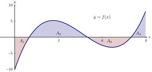
_images/int_neg.png — Fig. 37 Negative and positive values of integral#

Fact

The sign of the integral changes when the limits of the intergration are reversed

\[ \int_{a}^{b} f(x) dx = -\int_{b}^{a} f(x) dx \]

The fundamental theorem of calculus#

Direct connection between indefinite and definite integrals

Integral with varying upper limit#

Fact

Let \(f(x)\) be a continuous function on \([a,b] \subset \mathbb{R}\). Define the function \(\phi: [a,b] \to \mathbb{R}\) as

\[ \phi(t) = \int_a^t f(x) dx \]

\(\phi(t)\) has the following properties:

\(\phi(t)\) is continuous on \((a,b]\)
\(\phi(t) \to 0\) as \(t \to a\)
for all \(t \in (a,b)\) the derivative of \(\phi(t)\) is defined and given by \(\phi'(t) = f(t)\)

it follows that \(\phi\) is an anti-derivative of \(f\)
therefore, every continuous function has an anti-derivative
even when it is impossible to find a simple formula for the anti-derivative

Newton-Leibniz formula#

Fact (Fundamental theorem of calculus)

Let \(f(x)\) be a continuous function on \([a,b] \subset \mathbb{R}\) and \(F(x)\) is its anti-derivative on \([a,b]\). Then

\[ \int f(x) dx = F(x) + C \quad \implies \quad \int_a^b f(x) dx = F(b)-F(a) \]

Proof

Consider the function \(\phi(t) = \int_a^t f(x) dx\), then it is an anti-derivative of \(f\) on \([a,b]\) by the previous fact, i.e. \(F(x) = \phi(x) +C\). We have \(\phi(a) = 0\) and \(\phi(b) = \int_a^b f(x) dx\) (by definition of \(\phi\)). Then

\[ F(b)-F(a) = \phi(b) - \phi(a) = \int_a^b f(x) dx -0 = \int_a^b f(x) dx \]

\(\blacksquare\)

We aslo use notation

\[ F(x)\Big|_a^b = \Big|_a^b F(x) = F(b) - F(a) \]

Example

\[ \int_0^1 x^2 dx = \frac{x^3}{3}\Big|_0^1 = \frac{1}{3} -\frac{0}{3} = \frac{1}{3} \]

\[ \int_0^1 \exp(x) dx = \exp(x)\Big|_0^1 = \exp(1) - \exp(0) = e-1 \]

Infinite integration limits#

We can use the integral with the varying upper limit to extend the definition of the integral to infinite limits

Definition

The integral with infinite upper bound exists if the corresponding limit of the integral with the varying upper bound exists

\[ \int_{a}^{\infty} f(x) dx=\lim_{b \to \infty} \int_{a}^{b} f(x) dx \]

Similarly, the integral with infinite lower bound exists if the corresponding limit of the integral with the varying lower bound exists (varying lower bound is equivalent to varying upper bound with opposite sign of the integral)

\[ \int_{-\infty}^{b} f(x) dx=\lim_{a \to -\infty} \int_{a}^{b} f(x) dx \]

The integral with \([a,b] = [-\infty,\infty]\) is defined as

\[ \int_{-\infty}^{\infty} f(x) dx = \lim_{a \to -\infty} \int_{a}^{0} f(x) dx + \lim_{b \to \infty} \int_{0}^{b} f(x) dx \]

Example

\[ \int_1^\infty \frac{1}{x^2} dx = \lim_{b \to \infty} \int_1^b \frac{1}{x^2} dx = \lim_{b \to \infty} \left(-\frac{1}{x}\Big|_1^b\right) = \lim_{b \to \infty} \left(1-\frac{1}{b}\Big|_1^b\right) = 1 \]

a lot of the times Newton-Leibniz formula applies “directly” wihotuh having to think too much about the limit
the integrals of this type appear a lot in probability theory
watch the great video on Gaussian integral by 3Blue1Brown

Integration techniques#

The main difference from the techniques applied for the indefinite integrals is that we need to be careful with the limits of integration

Fact (Change of variables in definite integrals)

Suppose that \(f: [a,b] \to \mathbb{R}\) is integrable on \([a,b]\) and let \(\omega : \Omega \to [a,b]\), where \(\Omega \subseteq \mathbb{R}\), be a differentiable function with well-defined inverse. Then:

\[ \int_a^b f(x) dx = \int_{\omega^{-1}(a)}^{\omega^{-1}(b)} f(\omega(t)) \omega^{\prime}(t) dt \]

Example

\[ \int_{1}^2 x^3\sqrt{1+x^2} dx = \]

Let \(t=\omega^{-1}(x)=\sqrt{1+x^2}\), \(t\ge 1\), then \(x=\omega(t)=\sqrt{t^2-1}\) and \(\omega'(t) =\frac{t}{\sqrt{t^2-1}}\). The limits change as \(\omega^{-1}(1) = \sqrt{1+1}\), \(\omega^{-1}(2) = \sqrt{1+4}\). Continueing the derivation

\[ = \int_{\sqrt{2}}^{\sqrt{5}} \left(\sqrt{t^2-1}\right)^3 t \frac{t}{\sqrt{t^2-1}} dt = \int_{\sqrt{2}}^{\sqrt{5}} (t^2-1) t^2 dt = \]

\[ = \int_{\sqrt{2}}^{\sqrt{5}} (t^4 - t^2) dt = \left(\frac{1}{5}t^5 - \frac{1}{3}t^3 \right) \Big|_{\sqrt{2}}^{\sqrt{5}} = \frac{1}{5}5^{\frac{5}{2}} - \frac{1}{3}5^{\frac{3}{2}} - \frac{1}{5}2^{\frac{5}{2}} + \frac{1}{3}2^{\frac{3}{2}} \]

Fact (Integration by part in definite integrals)

Suppose that \(u,v: [a,b] \to \mathbb{R}\) is integrable on \([a,b]\), where \([a,b] \subseteq \mathbb{R}\) is a connected interval. Then

\[ \int_a^b u'(x) v(x) dx = u(x) v(x) \Big|_a^b - \int_a^b v'(x) u(x) dx \]

Example

\[ \int_{-a}^a x \exp(x) dx = \]

Let \(u(x)=\exp(x)\), \(v(x)=x\), then \(u'(x)=\exp(x)\), \(v'(x)=1\)

\[ = x \exp(x) \Big|_{-a}^a - \int_{-a}^a \exp(x) dx = a\left(e^a + \frac{1}{e^a} \right) - \exp(x) \Big|_{-a}^a = \]

\[ = a\left(e^a + \frac{1}{e^a} \right) - e^a + \frac{1}{e^a} = (a-1)e^a + \frac{a+1}{e^a} \]

Differentiating definite integrals#

Consider a definite integral as a function of some parameter variable \(t\). We assume that both the integrand and the limits of integration are functions of \(t\)

\[ I(t)=\int_{a(t)}^{b(t)} f(x,t) dx \]

Fact (Leibniz’ Rule)

For a well-defined integral with parameter \(t\) it holds

\[ \frac{d I(t)}{dt}= f\big(b(t),t\big) b^{\prime}(t)-f\big(a(t),t\big) a^{\prime}(t)+ \int_{a(t)}^{b(t)} \frac{\partial f(x,t)}{\partial t} dx \]

where \(a'(t)\) and \(b'(t)\) are the derivatives of the limits of integration with respect to \(t\)

note how Leibnitz rule is a generalization of the integral with varying upper limit

We may consider some special sub-cases of Leibniz’ rule:

\(a(t)\) and \(b(t)\) are functions of \(t\), but \(f(x)\) is not a function of \(t\). Here we have:

\[ \frac{d I(t)}{dt}=f\big(b(t), t \big) b^{\prime}(t)-f\big(a(t),t\big) a^{\prime}(t) \]

\(f(x)\) is a function of \(t\), but \(a\) and \(b\) are not functions of \(t\). Here we have:

\[ \frac{d I(t)}{dt}=\int_{a}^{b} \frac{\partial f(x, t)}{\partial t} dx \]

Example

Consider a function \(g(t)\) defined as

Derivative of this function can be found directly

\[ g(t) = \int_{0}^{t} \sqrt{x + t} dx = \frac{2}{3} (x + t)^{3/2} \Big|_0^t = \frac{2}{3} [(2t)^{3/2} - t^{3/2}] = \frac{2}{3} (2\sqrt{2}-1) t^{3/2} \]

\[ g'(t) = (2\sqrt{2}-1) \sqrt{t} \]

Or using the Leibniz rule

\[ g'(t) = \sqrt{2t} + \int_{0}^{t} \frac{dx}{2 \sqrt{x+1}} = \sqrt{2t} + \frac{1}{2} 2\sqrt{x+t} \Big|_0^t = \sqrt{2t} + \sqrt{2t} - \sqrt{t} = (2\sqrt{2}-1) \sqrt{t} \]

Some economic and econometric applications#

Consumer Welfare: Total Consumer Benefit, Consumer Surplus and Change in Consumer Surplus
Producer Welfare: Total Operating Costs, Producers Surplus, and Change in Producers Surplus
Choice over Time: Lifetime Utility
Choice under Uncertainty: Expected Utility
The Relationship between Probability Density Functions and Cumulative Distribution Functions (Probability and statistics)
The Expected Value and Other Moments of a Probability Distribution (Probability and statistics)
The Moment Generating Function and the Characteristic Function (Probability and statistics)

Preferences over time contingent consumption#

Consider a consumer that must choose how to allocate their lifetime wealth over consumption at various points in time

If time is continuous over some interval \([0, T]\) and the consumer can potentially consume at every point in time \(t \in[0, T]\), then a time-stream of consumption is a function of the form \(c:[0, T] \to[0, \infty)\). This function specifies, for each point in time \(t \in[0, T]\), the amount of consumption \(c(t) \in[0, \infty)\) that is chosen by the consumer (at time zero) for the point in time \(t \in[0, T]\)

In such cases, we sometimes assume (at least partly for tractability reasons) that such a consumer’s preferences over alternative consumption streams can be represented by a stationary “lifetime utility function” of the form

\[ U\left(\{c(t)\}_{t \in[0, T]}\right)=\int_{0}^{T} u(c(t)) e^{-\rho t} d t \]

where \(\rho \in(0,1)\) is a fixed rate of time preference and \(u(c)\) is a stationary per-period (or point-in-time) utility function

Preferences over state contingent consumption#

Suppose that there are an uncountably infinite number of potential states of the world, with each point in the interval non-empty closed interval \((a, b)\) corresponding to a particular state. Denote the state variable by \(\omega \in[a, b]\)

Nature chooses which state of nature will actually prevail by drawing one state from \((a, b)\) according to a commonly known probability distribution that has a probability density function of the form \(f:(a, b) \to[0,1]\)

Suppose that a consumer’s consumption level varies with the random state of Nature, so that it is given by a function of the form \(c:(a, b) \to[0, \infty)\)

If the consumer is a von Neumann-Morgenstern (vNM) expected utility maximiser with a Bernoulli utility function \(u:[0, \infty] \to \mathbb{R}\) of the form \(u(c)\), then the “vNM expected utility function” for this consumer is

\[ U\left(\{c(\omega)\}_{\omega \in[a, b]}\right)=\int_{a}^{b} u(c(\omega)) f(\omega) d \omega \]

Notes from the lecture#

Hand written notes from the lecture

📖 Univariate integration

Contents

📖 Univariate integration#

Anti-derivative#

Anti-derivatives are NOT unique#

Indefinite integral#

Properties of indefinite integral#

Integration zoo#

Integration techniques#

Direct integration#

Integration by substitution#

Integration by parts#

Definite integral#

Negative values of integrals#

The fundamental theorem of calculus#

Integral with varying upper limit#

Newton-Leibniz formula#

Infinite integration limits#

Integration techniques#

Differentiating definite integrals#

Some economic and econometric applications#

Preferences over time contingent consumption#

Preferences over state contingent consumption#

Notes from the lecture#